Introduction
Machine Learning is not a robot unlike most people perceive. Machine Learning is the science (art) of programming that gives computers the ability to learn from data without being explicitly programmed. It has been around for decades in many fields. But the first breakthrough of ML improving the lives of many people was the spam filter developed back in the 1990s. Since then, it has been applied for hundreds of applications including medical science and health, engineering and audio recognition and so on.
Machine Learning is a specific subfield of Artificial Intelligence that looks at the human brain’s architecture on how to build an intelligent machine. This is the key idea for Artificial Intelligence but it have gradually become quite different from their biological analogy.
Artificial Intelligence is the very core of Deep Learning. In comparison with Artificial Intelligence, Deep Learning usually involves much more successive layers of representations. It is a major field of Machine Learning for tackling very complex problems that Machine Learning is unable to resolve such as classifying billions of images, speech recognition, computer vision. Deep Learning requires big data in order to receive higher performance than Machine Learning and Artificial Intelligence.
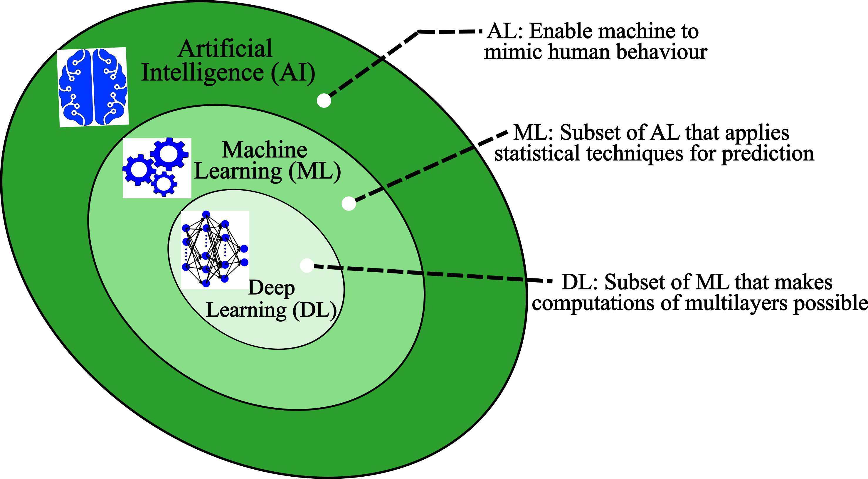
Many people use the words Artificial Intelligence, Machine Learning and Deep Learning interchangeably. But you can see there is clear difference in the Figure above.
Traditional Programming vs. Machine Learning
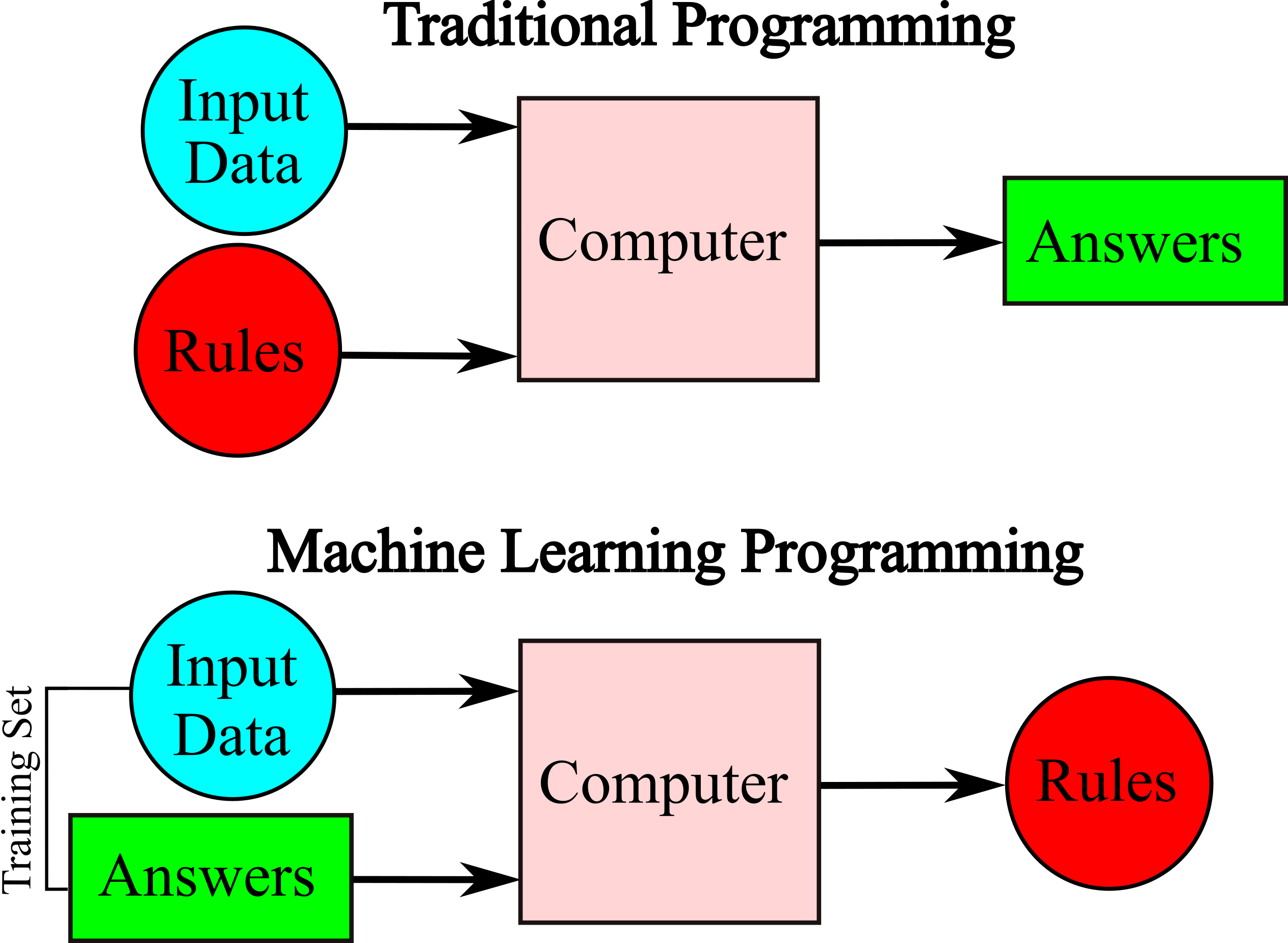
Traditional Programing: Programmers or software developers create programs that specify how to transform input data into the desired answer based on some predefined rules. For example, for writing a spam filter:
1- you should know what key phrases or words can be related to spam for example “amazing”, “for U”, ”free”, “credit card" may be often seen in the subject or a few other patterns in the body of email.
2- for each pattern or key word, you should write a detection algorithm to flag emails as spam.
The steps of 1 to 2 are repeated many times until to reach an acceptable prediction. This process is not simple and the code will have a long list of complicated rules. If spammers understand that “for U” emails are blocked, they might replace it with “For you”. Then, your code for filtering spam should be updated to flag “For you” emails. Writing new rules can go forever!
Moreover, there are some problems that are very complex or without known algorithm. For example, distinguishing the words “three” and “four” (speech recognition). It might be possible to hardcode an algorithm. However, this technique may not be efficient in case of thousands of words spoken by millions of people. The best solution is to write an algorithm that learns by itself by giving many recording examples.
Machine Learning: Programmers create appropriate models that can automatically learn to generate the desired answer for given input data. Machine Learning techniques for a spam filter automatically learns which phrases and words are predictors of spam by detecting unusually frequent patterns of words in the spam examples. The program is much easier and shorter to maintain, and most likely more accurate. The complex rules are not required, only need many examples of input data (emails) and answer (spam or not spam).The examples that the system uses to learn are called the training set. Each training example is called a training instance (or sample).
Types of Predictive Machine Learning
There are many different categories of machine learning. The most important areas depending on human supervision are supervised, unsupervised and semisupervised learning
Supervised Learning
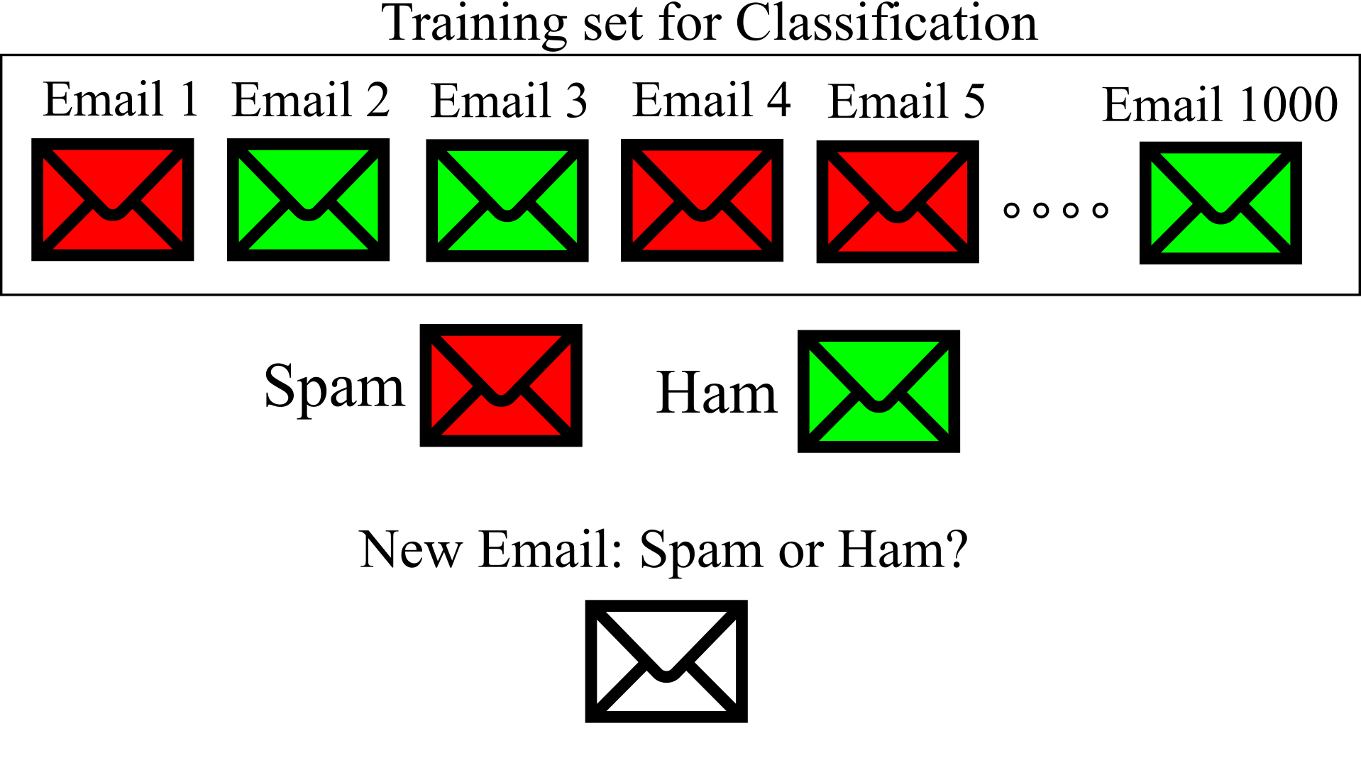
The training data for machine learning algorithm has a desired answer (solution), called labels. The figure below shows training set of supervised learning for Spam filter. There are 1000 emails and each email has a label as Spam or not Spam. Supervised learning task can be divided to 1- Cassification and 2- Regression. The Spam filter is an example of classification: many emails with their class (Spam or Ham) are used for training a model that learn how to classify new emails as Spam or Ham.
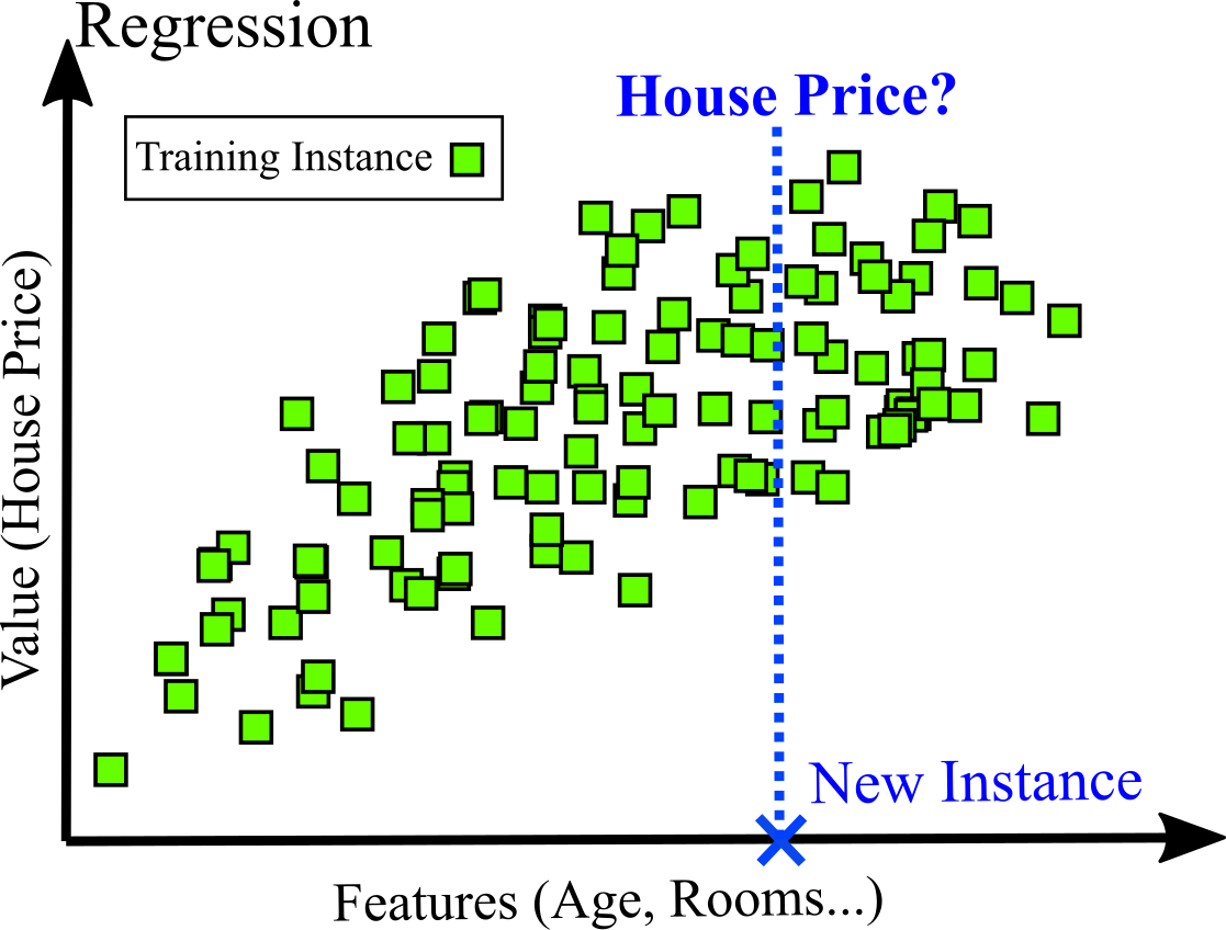
Another typical task is to predict a target numeric value, such as the price of a house, based a set of features such as location, age, number of rooms... This is a regression task. For training, many examples of houses, including both their features and their labels (prices) are required. An attribute in Machine Learning is a data type (e.g., “age”), while a feature has several meanings, but generally means an attribute along with its value (“age =10 years”). Figure belows shows an example of regression task.
Unsupervised Learning
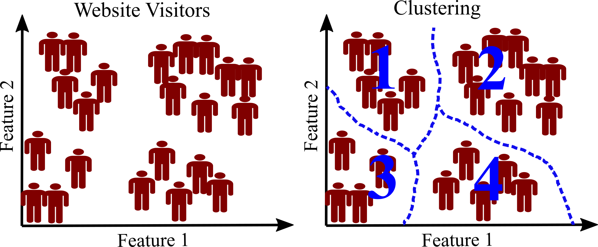
The training data in unsupervised learning has no label. Learning is done without a teacher. The most important unsupervised learning algorithms are 1- Clustering: a simple example is visitors of a website. Clustering algorithm can be applied to detect groups of similar visitors. The algorithm does not know which group belongs to a visitor. The connections are achieved without human supervision. For example, the result of clustering may show that 60\% of website visitors are males who read the website in the morning (see figure below).
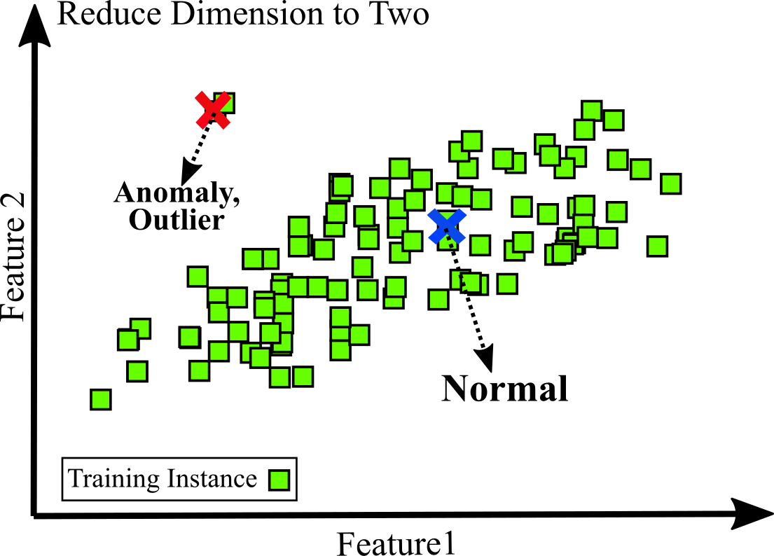
2- Dimensionality reduction: dimensionality reduction is a good example of unsupervised learning algorithms. If there are a lot of complex and unlabeled with many features, dimensionality reduction can be applied to reduce features to most important 2 or 3 features. Then, 2D or 3D representation of data can easily be plotted. This data visualization can leads to anomaly (outlier) detection. For example, preventing fraud or detecting unusual credit card transactions, catching manufacturing defects (see Figure below). A very similar task is novelty detection: the difference is that only normal data are expected to see during training (assumed there is no outlier in training set).
Semisupervised Learning
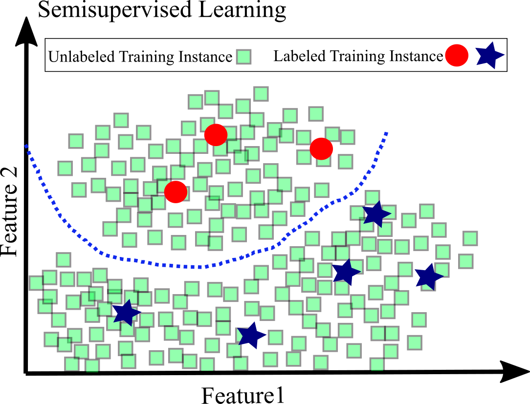
Labeling data is usually expensive and time-consuming. If there are a lot of unlabeled data and a little labeled data is available, semisupervised learning can be applied; it is a combination of unsupervised and supervised algorithms. For example, if we have many images of handwritten digits, but only a few images have labels. First clustering algorithm is applied to detect groups of similar images. Now the system only requires from human supervision to tell which digit can be assigned to each group using the few labeled data. This approach make it possible to predict the digit for each image using only a few labeled data.
Types of Learning: Instance-Based Versus Model-Based
Machine Learning systems can be categorized by how they generalize. As discussed above, making predictions are the most Machine Learning tasks. This signifies that by feeding a number of training examples, the system should be capable of generalizing to examples it has never seen before. We may have a good performance on the training data; however, the main goal is to perform well on new instances. There are two main generalization techniques: instance-based learning and model-based learning.
Instance-based learning:
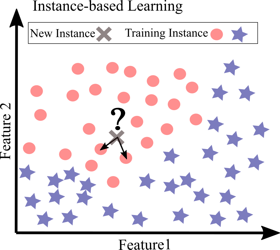
Learning by heart is possibly the most trivial form of learning. For spam filter task, we can flag all emails that are similar to the emails that have already been flagged as spam; however; this may not be an efficient solution. This approach called instance-based learning: the system learns everything by heart, then by using a similarity measurement, it generalizes to new cases by comparing them to the learned examples. Figure below shows an example of instance-based learning. The new instance is classified as a circle since the most similar instances belong to this class.
Model-based learning:
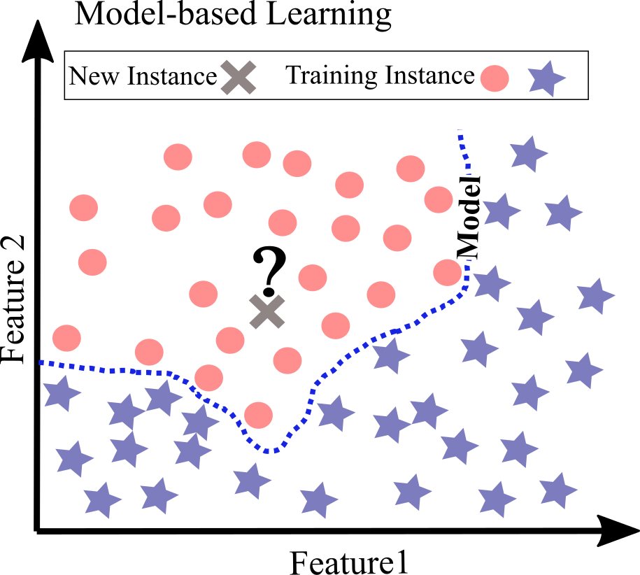
Model-based learning is another way to generalize from a set of examples; it fits the best model to the examples; this model is used for predictions. For example in Figure below, after fitting a model (dashed line), the new instance belongs to the circle class.
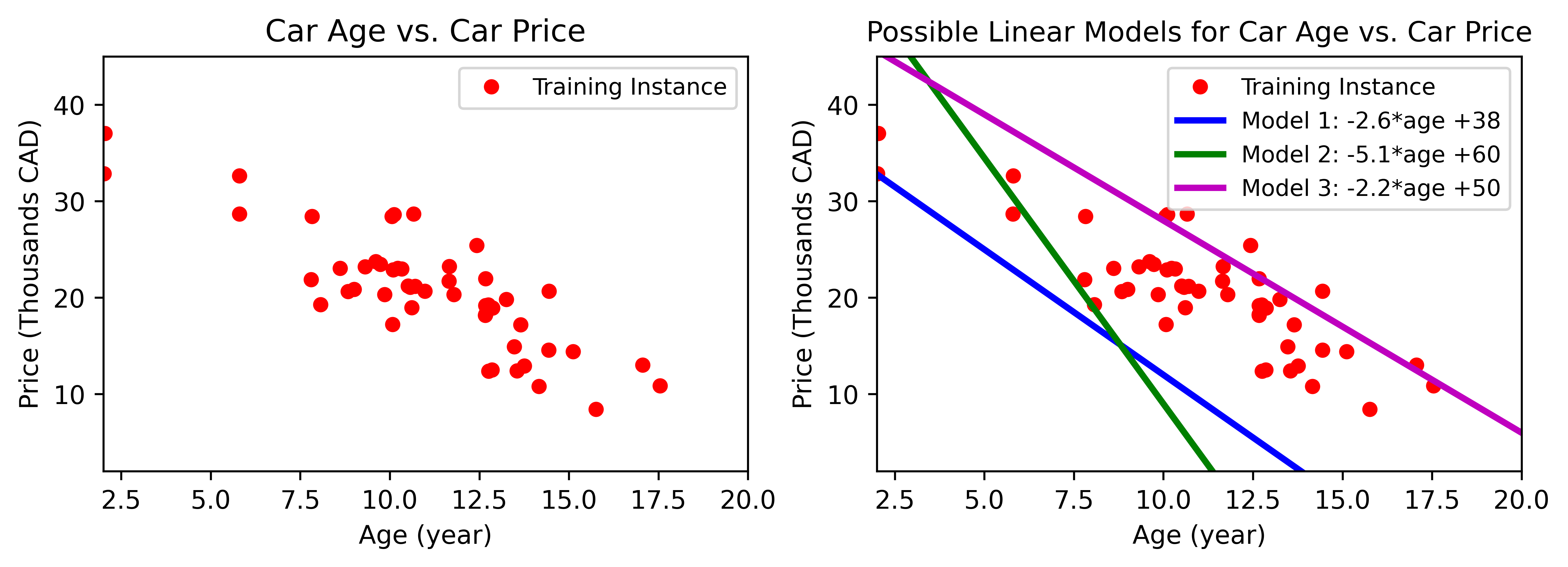
Another synthetic example is car price versus the age for 100 used cars shown in Figure below. Although the data is noisy, there is a linear trend (negative) between the age and price. By increasing age, car price seems to go down. We want to model car price as a linear function of age; this step is called model selection $Car\,price = w_{1} × age+w_{0}$. There are two parameters for this model, $w_{0}$ and $w_{1}$. Any linear function can be achieved by tweaking these parameters (Figure below).
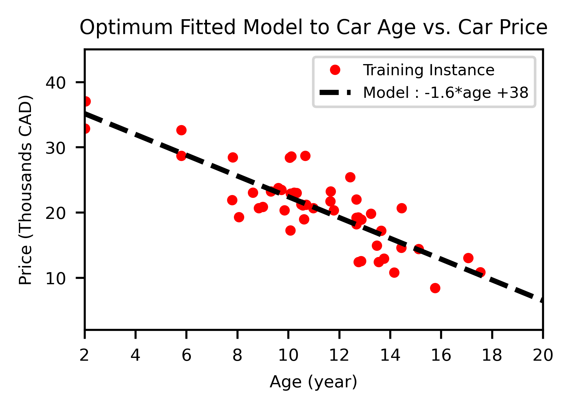
Using this model requires to define optimum values for the parameter $w_{0}$ and $w_{1}$. The optimization requires performance measurement that signifies how good your model or how bad your model is. Usually a Cost Function is applied to measure how bad a model is. By minimizing the cost function, the best linear model is fit to the data. This process is called training the model. The optimum parameter for Car price example are $w_{1}=-1.6$ and $w_{0}=38$: $Car\,price = -1.6 × age+38$. This simple model now can be used to make prediction.
To recap:
1- Study data and select a model (linear or not linear).
2- Train the model on the training data for example find optimum parameters to minimize a cost function.
3- Apply the model for to make predictions on new cases assuming that the model generalize data well.
Machine Learning Challenges
Limited Training Data
Machine Learning algorithms usually needs a lot of data to work properly and get high performance. Sometimes, thousands examples requires even for a simple problem, and millions of examples for complex problems such as speech or image recognition. However, this is a very common problem since it is not always possible to get extra expensive training data.
Non-representative Training Data
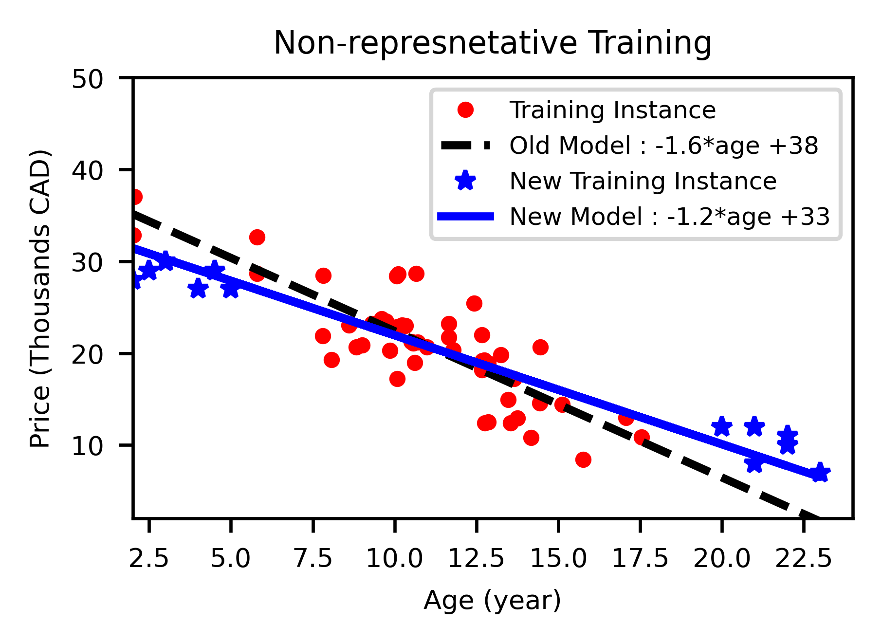
Sometime there are a large quantity of data; but machine learning algorithm cannot generalize well because the training data set is not representative of new cases. For example, the data set of car price was not perfectly representative; some key data were missing (stars). The dashed line is fitted on old data set and solid line is fitted on all data including new instances. As it can be seen, the new model changes significantly by instances, so old model is probably never work well, probably makes inaccurate predictions. This flawed sampling approach is called sampling bias. A famous example of sampling bias happened during the US presidential election in 1936, Landon against Roosevelt. A very large poll was conducted by sending mails to about 10 million people and receiving 2.4 million answers, it was predicted that Landon with high confidence would win the election. But, Roosevelt won the election due to sampling method:
1- The addresses of people for sending the polls was obtained from lists of magazine subscribers, telephone directories, club membership lists, and so on. All of these lists includes rich people that were more likely to vote Republican (Landon).
2- From those people who received the poll, less than 25% answered. Again, this introduces a sampling bias, that shows people who don’t care much about politics, and/or don’t like the polling company. This is a special type of sampling bias called nonresponse bias Aurélien Géron, 2019.
Low Quality of Training Data
Detecting the underlying patterns for the system is very tough if the training set has a lot of outliers, noise and error. Thereby, it is essential to spend some time and effort for cleaning the training data. If there are missing values, there should be reasonably imputed. Most data scientist spend a lot of time on this step.
Irrelevant Features in Training Data
If there are many irrelevant features, the system can not learn well because the irrelevant features hide patterns and trends in training Data. A very important part of Machine Learning project to have high performance is to select a good set of features. This step is called feature engineering includes 1- Feature selection: selecting the most important features to train, 2- Feature extraction: integrating existing features to generate a more practical one. 3- Gathering new data to create new features.
Overfitting the Training Data
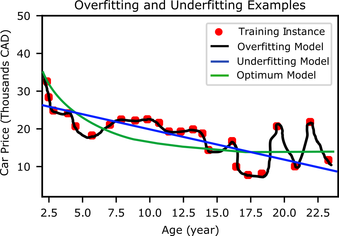
A simple example of overgeneralizing is when you are visiting a foreign country; you are charged a lot of money whenever you go to any restaurant. In this case, you are tempted to say all restaurant owners in that foreign country are thieves: of course, this overgeneralizing is not true. Unfortunately, this phenomenon can occur in Machine Learning that is called overfitting. It means that the model's performance is very well on the training data, but it does not generalize data having low performance on new data set (never-before-seen data). Another example of overfitting: a student is studying very hard for an exam but instead of understanding concepts trying to memorize concepts in course materials. He/she receives a low grade in exam if questions are not exactly from course material. Figure below show an example of car price vs. age in case of nonlinear correlation. Overfitting is a high-degree polynomial model that strongly overfits the training data. Despite it performs very well on training, it should give very low performance for new instances. Complex models including deep learning can detect patterns in the data, but if there are small noises in the training set, then the model is likely to detect patterns in the noise itself: these patterns cannot be seen for new instances. To avoid overfitting; 1- Simplify the model by selecting fewer parameters (reduce degree of polynomial model) or by constraining the model (regularization) or decrease number of features; 2- Remove noise, outliers and artifacts from taring data 3- Gather more training data.
Underfitting the Training Data
Underfitting happens when the model is too simple to learn the underlying pattern and structure of the data: it is the opposite of overfitting. Figure above shows a schematic illustration of overfitting and underfitting for a car price vs. age. A linear model (blue line) is underfitting; in reality, the model should be more complex than the linear model. On the other hand, high-degree polynomial model (black line) is overfitting detecting noises in data as patterns. To void underfitting: 1- Choose a more powerful model, with more parameters, 2- Apply feature engineering to feed better features to the algorithm, 3- Decrease applied the constraints for the model (regularization parameters).
