Introduction
Decision Trees is a powerful algorithms that can be applied for both classification and regression tasks. Decision Trees is among the most versatile and reliable machine learning algorithms for non-linear and complex data. Decision Trees is the fundamental component of Random Forest that will be discussed next lecture. Decision Trees is applied based on a flowchart structure. We start by generating a synthetic example with two classes; details about training, prediction and limitation of this technique are presented.
Generate Synthetic Data (Moons Dataset)
The following code shows how to generate a synthetic data set using make_moons that makes two interleaving half circles:
import pandas as pd
import numpy as np
import matplotlib
import pylab as plt
from numpy import random
from sklearn.datasets import make_moons


font = {'size'   : 12}
matplotlib.rc('font', **font)
fig = plt.subplots(figsize=(6.0, 4.5), dpi= 90, facecolor='w', edgecolor='k')

X, y = make_moons(n_samples=1000, noise=0.42, random_state=85)
X1=X[:,0] ; X2=X[:,1]
ik=0; ind=[]
for j in X2:
    if(y[ik]==0):
        if X1[ik]<-0.2:
            ind.append(ik)
        elif(j>-0.1):
            ind.append(ik)
    elif(y[ik]==1):
        if(j<-0.0):
            ind.append(ik)
    ik+=1

X1=X1[ind] ; X2=X2[ind]; y=y[ind]

random.seed(42)
x_1=random.randint(-15,-5,100)/10
x_2=random.randint(-15,1,100)/10
y_1=random.randint(0,1,100)

X1=np.concatenate((X1,x_1),axis=0)
X2=np.concatenate((X2,x_2),axis=0)
y=np.concatenate((y,y_1),axis=0)
def moon_dataset(X1,X2, y, axes):
    plt.plot(X1[y==0], X2[y==0], "bs", label="Class 0")
    plt.plot(X1[y==1], X2[y==1], "r^", label="Class 1")
    plt.xlabel(r"$X_{1}$", fontsize=18)
    plt.ylabel(r"$X_{2}$", fontsize=18, rotation=0)
    plt.grid(True, which='both')
    plt.axis(axes)
    plt.legend(loc="lower right", fontsize=14)

moon_dataset(X1,X2, y, [-1.5, 3, -1.5, 2])

plt.title('Synthetic Dataset with Two Classes', fontsize=18)

a=np.array(X1)
b=np.array(X2)
a=a.reshape(len(X1),1)
b=b.reshape(len(X2),1)
X=np.concatenate((a,b),axis=1)

plt.show()

Decision Trees
A Decision Trees model is trained with the moon dataset using DecisionTreeClassifier
from sklearn.tree import DecisionTreeClassifier

np.random.seed(42)
tree_clf = DecisionTreeClassifier(max_depth=2)
tree_clf.fit(X, y)
# Predict the fist 5 instances
tree_clf.predict(X[:5])
# The actual 5 instances
y[:5]
from sklearn.model_selection import cross_val_score

Accuracies=cross_val_score(tree_clf,X,y, cv=4, scoring="accuracy")
Accuracies
The trained Decision Tree can be visualized by first using the export_graphviz() method to output a graph definition file DecisionTrees.dot and use the "dot -Tps DecisionTrees.dot -o DecisionTrees.eps" to convert dot file to a eps picture. See the following code.
# Plot Decision Trees for flow chart

from sklearn.tree import export_graphviz
import os

export_graphviz(tree_clf,out_file="DecisionTrees.dot",
                feature_names=['X1','X2'],
                class_names=['0','1'],rounded=True,filled=True)

command = "dot -Tps DecisionTrees.dot -o DecisionTrees.eps"
os.system(command)
plt.show()
The Figure below shows visualization for trained Decision Tree with moon dataset.
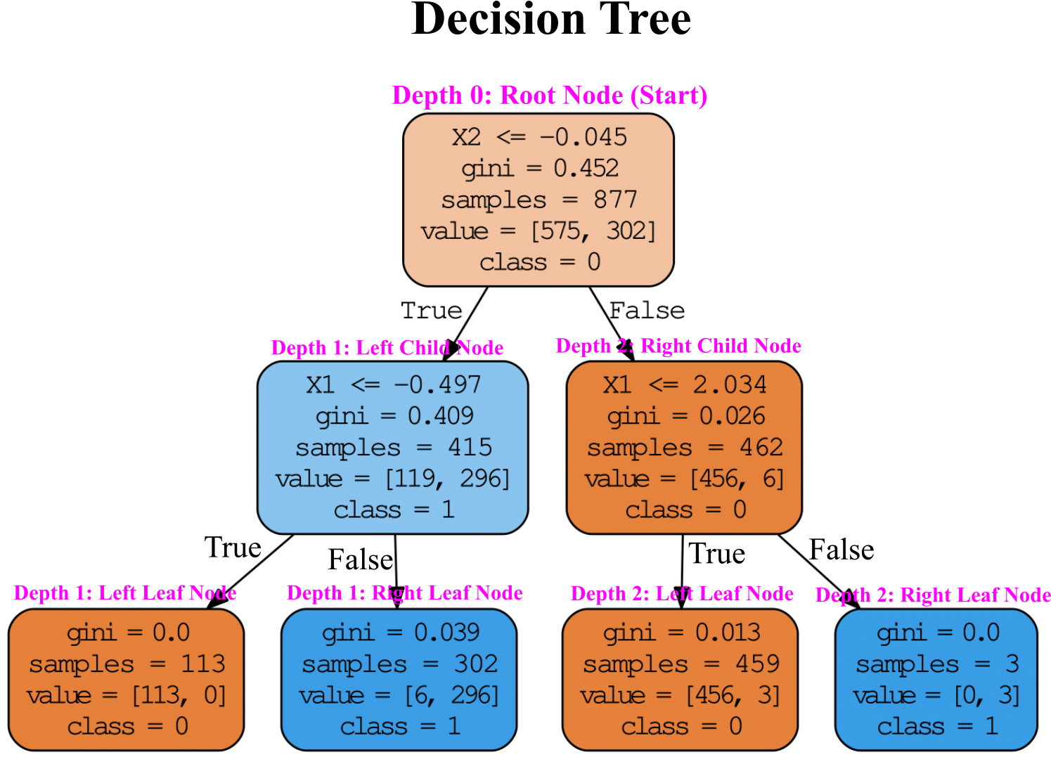
Root Node (Start)
Let’s see how the tree represented in Figure above makes predictions. We start at the Root Node (Depth 0): this node asks whether the $X\leqslant-0.045$. If it is, then you move down to the root’s left Child Node (Depth 1). If not, it goes to the root’s right child node (Depth 1). A Leaf Node does not have any children nodes, so it does not ask any questions (see left and right Leaf Nodes in Figure above).
For each node, gini attribute measures the impurity: a node is “pure” (gini=0) if we have all the training instances belong to the same class.
The equation below shows how to compute the gini score:
$gini=1-\sum_{k=1}^{n} P_{k}^{2}$
$P_{k}$ is the ratio of class k instances among the training instances for each node. For example the gini score for the Root Node (Depth 0) is $1-(\frac{575}{877})^{2}-(\frac{302}{877})^{2}=0.452$
The gini reduces from Root Node to Leaf Node, so the predicted class is based on Leaf Node. The following codes shows how to calculate gini for each node:
X_p=X.reshape(len(X1),2)
y_p=y.reshape(len(y),1)
x=np.concatenate((X_p,y_p),axis=1)
df=pd.DataFrame(x,columns=['X1','X2','y'])
df
def gini(x):
    val=1-sum([(i/sum(x))**2 for i in x])
    return np.round(val,3)
Result=df['y'].value_counts()
print('Total numbers=',sum(Result))
print('gini=',gini(Result))
print(Result)
Depth 1: Left Child Node
Result=df['y'][df['X2']<= -0.045].value_counts()
print('Total numbers=',sum(Result))
print('gini=',gini(Result))
print(Result)
Depth 1: Left Leaf Node
Result=df['y'][df['X2']<= -0.045][df['X1']<= -0.497].value_counts()
print('Total numbers=',sum(Result))
print('gini=',gini(Result))
print(Result)
Depth 1: Right Leaf Node
Result=df['y'][df['X2']<= -0.045][df['X1']> -0.497].value_counts()
print('Total numbers=',sum(Result))
print('gini=',gini(Result))
print(Result)
Depth 2: Right Child Node
Result=df['y'][df['X2']> -0.045].value_counts()
print('Total numbers=',sum(Result))
print('gini=',gini(Result))
print(Result)
Depth 2: Left Leaf Node
Result=df['y'][df['X2']> -0.045][df['X1']<= 2.034].value_counts()
print('Total numbers=',sum(Result))
print('gini=',gini(Result))
print(Result)
Depth 2: Right Leaf Node
Result=df['y'][df['X2']> -0.045][df['X1']> 2.034].value_counts()
print('Total numbers=',sum(Result))
print('gini=',gini(Result))
print(Result)
Figure below shows Decision Tree’s decision boundaries. The decision boundaries for depth=0 (the root node) is X2<= -0.045, for depth=1 is X1<= -0.497 and for depth=2 is X1<= 2.034.
from matplotlib.colors import ListedColormap
import matplotlib as mpl
import matplotlib.pyplot as plt

font = {'size'   : 12}
matplotlib.rc('font', **font)
fig = plt.subplots(figsize=(6.0, 4.5), dpi= 90, facecolor='w', edgecolor='k')

x1s = np.linspace(-1.8,3, 100)
x2s = np.linspace(-1.5,2, 100)
x1, x2 = np.meshgrid(x1s, x2s)
X_new = np.c_[x1.ravel(), x2.ravel()]
y_pred = tree_clf.predict(X_new).reshape(x1.shape)
custom_cmap = ListedColormap(['b','r'])
plt.contourf(x1, x2, y_pred, alpha=0.3, cmap=custom_cmap)
plt.plot(X[:, 0][y==0], X[:, 1][y==0], "bs", label="Class 0")
plt.plot(X[:, 0][y==1], X[:, 1][y==1], "r^", label="Class 1")

plt.axis([-1.5, 3, -1.5, 2])
plt.xlabel(r"$X_{1}$", fontsize=18)
plt.ylabel(r"$X_{2}$", fontsize=18, rotation=0)
plt.plot([-1.5, 3], [-0.045, -0.045], "k-", linewidth=2)
plt.text(0.6, 0.05, "Depth=0",style='oblique', ha='center',
         bbox=dict(facecolor='w', alpha=1,pad=0),
         va='top', wrap=True, fontsize=15)
#
plt.plot([-0.497, -0.497], [-1.5, -0.045], "k--", linewidth=2)
plt.text(-0.5, -0.75, "Depth=1",style='oblique', ha='center',
         bbox=dict(facecolor='w', alpha=1,pad=0),
         va='top', wrap=True, fontsize=15)
#
plt.plot([2.034, 2.034], [-0.045, 2.0], "k:", linewidth=2)
plt.text(2, 1, "Depth=2",style='oblique', ha='center',
         bbox=dict(facecolor='w', alpha=1,pad=0),
         va='top', wrap=True, fontsize=15)
plt.title('Decision Tree Decision Boundaries with max depth=2', fontsize=14)
plt.legend(loc=2, fontsize=14)
plt.show()

Regularization Hyperparameters
We saw in the Machine Learning main steps lecture that Decision Trees has greatly overfitted the training set. It was because all parameters have been freely selected. Decision Tree’s freedom can be restricted to avoid overfitting. As we mentioned before, this is called regularization. In Scikit-Learn, this is controlled by the max_depth hyperparameter (the default value for max_depth is unlimited). Reducing max_depth will reduce the risk of overfitting. Another hyperparameters are min_samples_leaf (the minimum number of samples a leaf node must have), max_leaf_nodes (maximum number of leaf nodes)... Reducing max or increasing min regularizes the model.
The Figure belows shows an overfitted model for max_depth=20 in left. In right Figure, we still have max_depth=20 but restrict min_samples_leaf to 5. This leads to avoid overfitting.
font = {'size'   : 12}
matplotlib.rc('font', **font)
fig = plt.subplots(figsize=(13.0, 4.5), dpi= 90, facecolor='w', edgecolor='k')

ax1=plt.subplot(1,2,1)
X, y = make_moons(n_samples=100, noise=0.42, random_state=85)

x1s = np.linspace(-1.8,3, 100)
x2s = np.linspace(-1.5,2, 100)
x1, x2 = np.meshgrid(x1s, x2s)
X_new = np.c_[x1.ravel(), x2.ravel()]
np.random.seed(42)
tree_clf = DecisionTreeClassifier(max_depth=2)
tree_clf.fit(X, y)
y_pred = tree_clf.predict(X_new).reshape(x1.shape)
custom_cmap = ListedColormap(['b','r'])
plt.contourf(x1, x2, y_pred, alpha=0.3, cmap=custom_cmap)
plt.plot(X[:, 0][y==0], X[:, 1][y==0], "bs", label="Class 0")
plt.plot(X[:, 0][y==1], X[:, 1][y==1], "r^", label="Class 1")

plt.axis([-1.5, 3, -1.5, 2])
plt.xlabel(r"$X_{1}$", fontsize=18)
plt.ylabel(r"$X_{2}$", fontsize=18, rotation=0)
plt.title("max_depth=20", fontsize=16)
plt.legend(loc=2, fontsize=14)

ax2=plt.subplot(1,2,2)

# Decision Trees
np.random.seed(42)
tree_clf = DecisionTreeClassifier(max_depth=20,min_samples_leaf=5)
tree_clf.fit(X, y)
y_pred = tree_clf.predict(X_new).reshape(x1.shape)
custom_cmap = ListedColormap(['b','r'])
plt.contourf(x1, x2, y_pred, alpha=0.3, cmap=custom_cmap)
plt.plot(X[:, 0][y==0], X[:, 1][y==0], "bs", label="Class 0")
plt.plot(X[:, 0][y==1], X[:, 1][y==1], "r^", label="Class 1")

plt.axis([-1.5, 3, -1.5, 2])
plt.xlabel(r"$X_{1}$", fontsize=18)
plt.ylabel(r"$X_{2}$", fontsize=18, rotation=0)
plt.title("max_depth=20 and min_samples_leaf=5", fontsize=16)
plt.legend(loc=2, fontsize=14)

plt.show()

Regression
Decision Trees can also be applied for regression task as we saw in Lecture 3 (for hydrocarbone production). Let’s build a regression tree for a synthetic data using Scikit-Learn’s DecisionTreeRegressor.
# Quadratic training set + noise
np.random.seed(52)
n = 100
X = np.random.rand(n, 1)
y =  10-(X-0.5) **2
y = y + np.random.randn(n, 1) / 15
from sklearn.tree import DecisionTreeRegressor

tree_reg = DecisionTreeRegressor(max_depth=2, random_state=42)
tree_reg.fit(X, y)
from sklearn.tree import DecisionTreeRegressor

font = {'size'   : 12}
matplotlib.rc('font', **font)
fig = plt.subplots(figsize=(13.0, 4.5), dpi= 90, facecolor='w', edgecolor='k')

ax1=plt.subplot(1,2,1)
reg_tree1 = DecisionTreeRegressor(random_state=20)
reg_tree1.fit(X, y)
x1 = np.linspace(0, 1, 500).reshape(-1, 1)
y_pred = reg_tree1.predict(x1)

plt.xlabel("$X$", fontsize=18)
plt.ylabel("$y$", fontsize=18, rotation=0)
plt.plot(X, y, "ro",markersize=6,label='Training Data')
plt.plot(x1, y_pred, "b-", linewidth=2, label='Fitted Model')
plt.title("max_depth=2", fontsize=16)
plt.legend(loc=4, fontsize=14)

ax2=plt.subplot(1,2,2)
reg_tree2 = DecisionTreeRegressor(random_state=20, max_depth=20)
reg_tree2.fit(X, y)
x1 = np.linspace(0, 1, 500).reshape(-1, 1)
y_pred = reg_tree2.predict(x1)

plt.xlabel("$X$", fontsize=18)
plt.ylabel("$y$", fontsize=18, rotation=0)
plt.plot(X, y, "ro",markersize=6,label='Training Data')
plt.plot(x1, y_pred, "b-", linewidth=2, label='Fitted Model')
plt.legend(loc=4, fontsize=14)
plt.title("max_depth=20 (overfitting)", fontsize=16)

plt.show()

Limitation of Decision Trees
We saw Decision Trees algorithm is simple, easy to use, and powerful. However, like every technique it has limitations. Decision Trees has orthogonal decision boundaries, which makes it difficult to fit training sets which require rotation. For example, the following code shows training Decision Trees model for synthetic orthogonal data in left and for 45° rotated training set in right. It seems both Decision Trees fit the training set well; but the model on the right does not generalize well.
np.random.seed(20)
Xs = np.random.rand(100, 2) - 0.5
ys = (Xs[:, 0] > 0).astype(np.float32) * 2
def rotate(x0,y0,x,y,Ang):
    """Rotate coordinate"""
    import math
    xa=[]
    ya=[]
    Angle=Ang *(math.pi/180)
    for i in range(len(x)):
        tmp1=x[i]-x0
        tmp2=y[i]-y0
        X=(tmp2)*math.sin(Angle)+(tmp1)*math.cos(Angle)
        xa.append(X+x0)
        Y=(tmp2)*math.cos(Angle)-(tmp1)*math.sin(Angle)
        ya.append(Y+y0)
    xa=np.array(xa).reshape(len(xa),1)
    ya=np.array(ya).reshape(len(ya),1)
    X=np.concatenate((xa,ya),axis=1)
    return X
font = {'size'   : 12}
matplotlib.rc('font', **font)
fig = plt.subplots(figsize=(13.0, 4.5), dpi= 90, facecolor='w', edgecolor='k')

np.random.seed(20)
X = np.random.rand(200, 2) - 0.5
y = np.array([1 if i > 0 else 0 for i in list(X[:, 0])])

ax1=plt.subplot(1,2,1)
X=rotate(0,0,X[:, 0],X[:, 1],-8)
x1s = np.linspace(-0.75,0.75, 100)
x2s = np.linspace(-0.75,0.75, 100)
x1, x2 = np.meshgrid(x1s, x2s)
X_new = np.c_[x1.ravel(), x2.ravel()]
np.random.seed(62)
tree_clf = DecisionTreeClassifier()
tree_clf.fit(X, y)
y_pred = tree_clf.predict(X_new).reshape(x1.shape)
custom_cmap = ListedColormap(['b','r'])
plt.contourf(x1, x2, y_pred, alpha=0.3, cmap=custom_cmap)
plt.plot(X[:, 0][y==0], X[:, 1][y==0], "bs", label="Class 0")
plt.plot(X[:, 0][y==1], X[:, 1][y==1], "r^", label="Class 1")

plt.xlabel(r"$X$", fontsize=18)
plt.ylabel(r"$y$", fontsize=18, rotation=0)
plt.title("Vertical Data", fontsize=16)
plt.legend(loc=2, fontsize=14)

ax2=plt.subplot(1,2,2)
X=rotate(0,0,X[:, 0],X[:, 1],45)
np.random.seed(62)
tree_clf = DecisionTreeClassifier(min_samples_leaf=3)
tree_clf.fit(X, y)
y_pred = tree_clf.predict(X_new).reshape(x1.shape)
custom_cmap = ListedColormap(['b','r'])
plt.contourf(x1, x2, y_pred, alpha=0.3, cmap=custom_cmap)
plt.plot(X[:, 0][y==0], X[:, 1][y==0], "bs", label="Class 0")
plt.plot(X[:, 0][y==1], X[:, 1][y==1], "r^", label="Class 1")

plt.xlabel(r"$X$", fontsize=18)
plt.ylabel(r"$y$", fontsize=18, rotation=0)
plt.title("Rotate Data for 45 Degree", fontsize=16)
plt.legend(loc=2, fontsize=14)
plt.show()

Energy Efficiency Data Set
import pandas as pd

df = pd.read_csv('Building_Heating_Load.csv',na_values=['NA','?',' '])
df[0:5]
df_binary=df.copy()
df_binary.drop(['Heating Load','Multi-Classes'], axis=1, inplace=True)
df_binary[0:5]
df_binary['Binary Classes']=df_binary['Binary Classes'].replace('Low Level', 0)
df_binary['Binary Classes']=df_binary['Binary Classes'].replace('High Level', 1)
df_binary[0:5]
import numpy as np

np.random.seed(32)
df_binary=df_binary.reindex(np.random.permutation(df_binary.index))
df_binary.reset_index(inplace=True, drop=True)
df_binary[0:10]
from sklearn.model_selection import StratifiedShuffleSplit

# Training and Test
spt = StratifiedShuffleSplit(n_splits=1, test_size=0.2, random_state=42)
for train_idx, test_idx in spt.split(df_binary, df_binary['Binary Classes']):
    train_set_strat = df_binary.loc[train_idx]
    test_set_strat  = df_binary.loc[test_idx]
# Note that drop() creates a copy and does not affect train_set_strat
X_train = train_set_strat.drop("Binary Classes", axis=1)
y_train = train_set_strat["Binary Classes"].values
from sklearn.preprocessing import StandardScaler

scaler = StandardScaler()
X_train=X_train.copy()
X_train_Std=scaler.fit_transform(X_train)
# Traning Data
X_train_Std[0:5]
np.random.seed(42)
tree_clf = DecisionTreeClassifier(max_depth=10,min_samples_split=5,min_samples_leaf=4)
tree_clf.fit(X_train_Std, y_train)
from sklearn.model_selection import cross_val_score

Accuracies=cross_val_score(tree_clf,X_train_Std, y_train, cv=4, scoring="accuracy")
Accuracies
from sklearn.model_selection import cross_val_predict
y_train_pred = cross_val_predict(tree_clf,X_train_Std,y_train, cv=4)
from sklearn.metrics import precision_score, recall_score

precision=precision_score(y_train, y_train_pred)
print('Precision= ',precision)

recall=recall_score(y_train, y_train_pred)
print('Recall (sensitivity)= ',recall)
Fine-Tune Your Model
Lets fine-tune hyperparameters of Descicion Trees max_depth,min_samples_leaf... with Scikit-Learn’ Grid Search and Randomized Search discussed in previous lecture.
Grid Search
from sklearn.model_selection import GridSearchCV

np.random.seed(42)
tree_clf = DecisionTreeClassifier()
params = {'max_depth': [2,5,10,20,30,40],'max_features': [2,3,4,5],'min_samples_leaf': [2,3,5,7]}

tree_search_cv = GridSearchCV(tree_clf, params, cv=5,scoring='recall')
tree_search_cv.fit(X_train,y_train)
tree_search_cv.best_params_
tree_search_cv.best_estimator_
cvreslt=tree_search_cv.cv_results_
cvreslt_params=[str(i) for i in cvreslt["params"]]
for mean_score, params in sorted(zip(cvreslt["mean_test_score"], cvreslt_params)):
    print(np.sqrt(mean_score), params)
Randomized Search
from sklearn.model_selection import RandomizedSearchCV
from scipy.stats import randint
import warnings
warnings.filterwarnings('ignore')

np.random.seed(42)
tree_clf = DecisionTreeClassifier()
params = {'max_depth': randint(low=2, high=30),'min_samples_leaf': randint(low=2, high=10)}

tree_search_cv = RandomizedSearchCV(tree_clf, params,n_iter=50, cv=5,scoring='recall')
tree_search_cv.fit(X_train,y_train)
tree_search_cv.best_params_
cvreslt=tree_search_cv.cv_results_
cvreslt_params=[str(i) for i in cvreslt["params"]]
for mean_score, params in sorted(zip(cvreslt["mean_test_score"], cvreslt_params)):
    print(np.sqrt(mean_score), params)