Introduction
In this lecture, first we will take a closer look at Linear Regression model that is one of the simplest model. Linear Regression will be trained by 1- computing directly the optimum model parameters to fit the training set (parameters that minimize cost function), 2- an iterative optimization approach, called Gradient Descent (GD), that gradually tweaks the model parameters to minimize the cost function reaching to the same set of parameters as the first method. Next, we will discuss about Polynomial Regression a more complex model that can fit nonlinear datasets. There is higher likelihood of overfitting for Polynomial Regression since it has more parameters than Linear Regression. Regularization technique will be discussed to reduce overfitting. Lastly, we will talk about Logistic Regression and Softmax Regression models that are commonly used for classification.
Linear Regression
In the first class, a simple regression model was shown for estimation of car price with the car age: $Car\,price = w_{0}+w_{1} × age$. This model is just a linear function of the input feature age. $w_{0}$ and $w_{1}$ are the model’s parameters. Making a prediction by a linear regression is simply applied by calculating a weighted sum of the input features, plus a constant called the bias term (intercept term): $y_{p}=w_{0}+w_{0}x_{0}+w_{1}x_{1}....+w_{n}x_{n}$ where $y_{p}$ is the predicted value, $n$ is number of features (age, type of car, millage, color...), $x_{j}$ is the $j^{th}$ feature value, $w_{j}$ is the $j^{th}$ model parameter (bias term $w_{0}$ and the feature weights $w_{1},w_{2},...,w_{n}$).
This can be written by using vectorized form: $y_{p}=\mathbf{w.x}$ where $\mathbf{w}$ is parameter vector of the model $w_{0},w_{1},w_{2},...,w_{n}$, and $\mathbf{x}$ is feature vectors including $x_{0},x_{1},x_{2},...,x_{n}$ with $x_{0}=1$.
The vectors are frequently shown as column vectors in Machine Learning; they are 2D arrays that have a single column. If $\mathbf{w}$ and $\mathbf{x}$ are column vectors, then for calculating $y_{p}$ we need to have transpose of $\mathbf{w}$ shown as $\mathbf{w^{T}}$ : $y_{p}=\mathbf{\mathbf{w^{T}}.\mathbf{x}}$; it is a matrix multiplication.
We explained Linear Regression, the problem is how to train the model to achieve optimum weights $w_{0},w_{1},w_{2},...,w_{n}$? We need to measure how bad (or good) the model fits the training data, called cost function. The most common cost function in Machine Learning is the Root Mean Square Error (RMSE) as we discussed before. The weights $w_{0},w_{1},w_{2},...,w_{n}$ should be defined to minimize the RMSE cost function
For doing this, we need to measure how bad (or good) the model fits the training data. We discussed in previous classes that the most common approach to measure performance of a regression model is the Root Mean Square Error (RMSE). So, to train a model, RMSE should be minimized to achieve optimum weights $w_{0},w_{1},w_{2},...,w_{n}$. It is easier to minimize the Mean Square Error (MSE) than the RMSE in practice: the results will be the same. If some weights minimize MSE, they for sure minimize RMSE.
$MSE=\frac{1}{n}\sum_{i=1}^{n}(\mathbf{\mathbf{w^{T}}.\mathbf{x^{i}}}-y^{i})^{2}$ where $n$ is number of data and $\mathbf{x^{i}}$ features (age, type of car, millage, color...) and $y^{i}$ is actual values. The main goal is to find the weights $\mathbf{w}$ that minimize $MSE$.
The Normal Equation
We can directly find optimum weights $\mathbf{w}$ to minimize $MSE$ by using Normal Equation:
$\mathbf{\bar{w}}=(\boldsymbol{X}^{T}\boldsymbol{X})^{-1} \boldsymbol{X}^{T} \boldsymbol{y}$ where $\mathbf{\bar{w}}$ is the vector of weights that minimize the cost function (MSE) and $\boldsymbol{y}$ is the vector of actual values.
See the following code to generate a synthetic data.
import numpy as np
import pylab as plt

np.random.seed(32)
X =3.5 * np.random.rand(200, 1) # Generate a Uniform distribution between 0 to 1.
y =5 + 2.5 * X + np.random.randn(200, 1) # Create a function and some Gaussian noise.
plt.plot(X,y,'ro')
plt.title("Synthetic Data with Linear Correlation",fontsize=15)
plt.xlabel("X",fontsize=15)
plt.ylabel("y",fontsize=15)
plt.show()
We want to calculate $\mathbf{\bar{w}}$ by The Normal Equation. We need to calculate Matrix Inverse (see $(\boldsymbol{X}^{T}\boldsymbol{X})^{-1}$ in Equation above). Inverse of a Matrix can be calculated with NumPy module:
X_ = np.c_[np.ones((200, 1)), X] # Generat 1 value 200 times and add to each instance
Opt_weight = np.linalg.inv(X_.T.dot(X_)).dot(X_.T).dot(y)
The optimum weights are:
print(' The calculated optimum weights with The Normal Equation are: \n')
print( 'w0: ', Opt_weight[0])
print( 'w1: ', Opt_weight[1])
The real function the we generate data was $y=2.5x$+5+some noise. We predicted the function $y=2.57x+4.89$: $w_{1}=2.57$ and $w_{0}=4.89$. It is close to real function but some added noise to the function make it impossible to achieve the same parameters. Now you can make prediction based on the achieved function. The following code shows how to predict the y values for x=0 and x=3.5 and connect two points as the predicted function.
New_X = np.array([[0], [3.5]])
New_X_= np.c_[np.ones((2, 1)), New_X] # Generat 1 value 2 times and add to each instance
predict_y = New_X_.dot(Opt_weight)
predict_y

plt.plot(X,y,'ro')
plt.plot(New_X,predict_y,'b-',linewidth=4)
plt.title("Synthetic Data and Fitted Linear Model",fontsize=15)
plt.xlabel("X",fontsize=15)
plt.ylabel("y",fontsize=15)
plt.show()
Applying Linear Regression in Scikit-Learn is quite simple as we saw before (for petroleum production prediction). Scikit-Learn uses Singular Value Decomposition (SVD)
from sklearn.linear_model import LinearRegression

lin_reg = LinearRegression()
lin_reg.fit(X, y)

print(' The calculated optimum weights with Scikit-Learn are: \n')
print( 'w0: ', lin_reg.intercept_)
print( 'w1: ', lin_reg.coef_[0])
You can simply make a Linear Regression prediction with Scikit-Learn:
lin_reg.predict(New_X)
Scikit-Learn does not use the Normal Equation. If the matrix is not invertible (for example singular matrix), the Normal Equation does not work. Scikit-Learn calculates the optimum weights by $\bar{\mathbf{w}}=\mathbf{X^{+}\mathbf{y}}$ where $\mathbf{X^{+}}$ is pseudoinverse of $\mathbf{X}$. Not every matrix has an inverse, but every matrix has a pseudoinverse: this approach can also handle singular matrix and it is more efficient than the Normal Equation.
However, both the Normal Equation and the pseudoinverse approach are very slow in case of large number of features. Now we will discuss a very different approach to train a Linear Regression model, that is capable of dealing with too many training instances and a large number of features to fit in memory (Aurélien Géron, 2019).
Gradient Descent
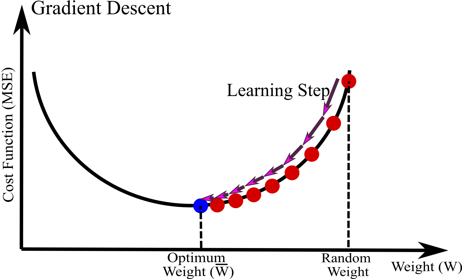
Gradient Descent is an optimization algorithm that can find optimal solutions for many problems. Generally, Gradient Descent tweak some parameters iteratively to minimize a cost function. A simple example how Gradient Descent works: imagine you are in the mountains and you face a very dense fog, you get lost and want to come back but you do not have any devices (GPS) to help to go downhill. You can only feel the slope of the ground below your feet. So, you can get to the bottom of the valley quickly if you go in the direction of the steepest slope. This is the main strategy of Gradient Descent: the gradient of the cost function with regards to the parameters $w$ is calculated; that leads to go in the direction of descending gradient. The equation below shows how Gradient Descent works:
$\Large w=w-\alpha \frac{\partial C}{\partial w}$
where $\frac{\partial C}{\partial w}$ is Gradient of cost function ($C$) with regards to weight $w$ and $\alpha$ is learning rate that will be discussed. By each iteration $w$ is updated and getting closer to downhill and finally reaching to the minimum of cost function when the gradient is zero that is when we will achieve optimum weight $\bar{\mathbf{w}}$.
Gradient Descent requires a random value for $w$ (random initialization); this random value is improved gradually decreasing the cost function (MSE). This process is repeated until the algorithm converges to a minimum cost function.
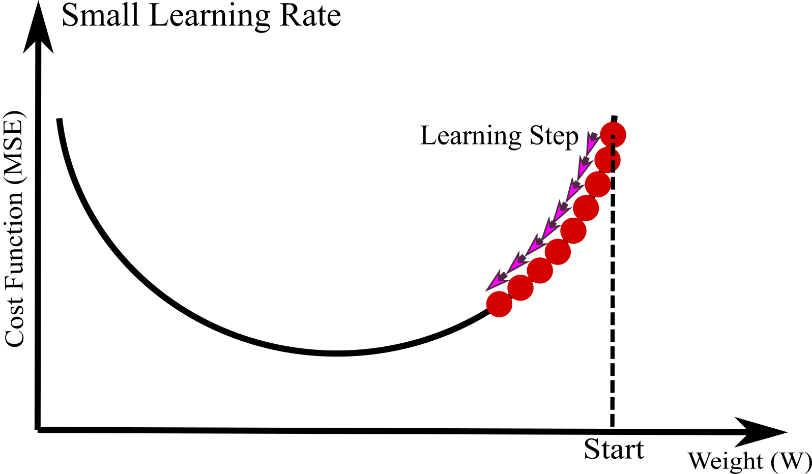
The size of learning step is very important in Gradient Descent, called learning rate hyperparameter. The algorithm will need many iterations to converge and reach global minimum if the learning is too small (see Figure below). The leads to take a long time which makes Machine Learning algorithm inefficient.
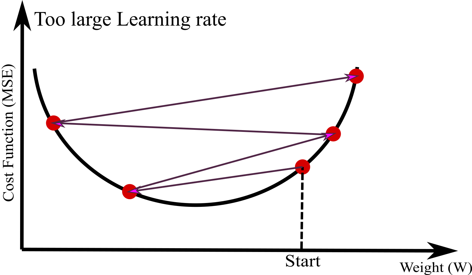
On the other hand, if you choose high learning rate, you could jump across the valley and go to the other side. This may lead to larger and larger cost function (algorithms diverges), failing to find the optimum weight.
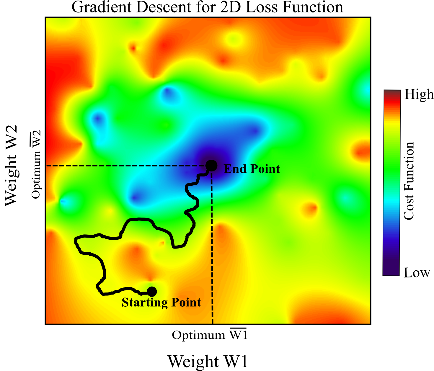
Last problem is all cost functions does not have a clear bowl shape. There may be ridges, holes, plateaus, making convergence to the minimum very difficult or impossible. Figure below shows the two main challenges with Gradient Descent: if the random weight starts from the right, then the algorithm should converge to a local minimum; however, it is not as efficient as the global minimum. If the random weight starts on the right, then the algorithm takes a very long time to pass the plateau: the global minimum cannot be met if the iteration stops too early.
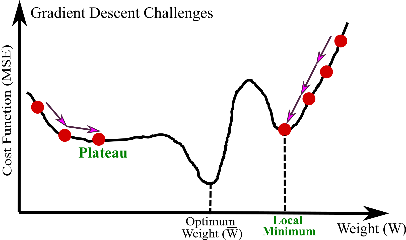
Figure below shows a 2D Gradient Descent. We start random initialization for weights $w_{1}$ and $w_{2}$ and find a way to go downhill of the calculated cost function. This approach can be applied for any number of weights. Gradient Descent requires training set to be standardized; otherwise, it takes much longer time to converge. If in Figure below, two features have different scales, one is much larger than another, then Gradient Descent algorithm cannot go straight toward the minimum.
Batch Gradient Descent
Implementation of Gradient Descent requires to calculate the gradient of the cost function with regards to the models parameters $w_{j}$. In fact, you need to know if you change $w_{j}$ a little, how much the cost function will change. Similar to asking the slope of mountain under your feet for different direction (East, North..). It is called partial derivative of the cost function (MSE) with regards to parameter $w_{j}$ written as $\frac{\partial }{\partial w_{j}} MSE (\mathbf{w})$:
$ \frac{\partial }{\partial w_{j}} MSE (\mathbf{w}) =\frac{2}{n}\sum_{i=1}^{n}(\mathbf{w}^{T}x^{i}-y^{i})x^{i}_{j}$
The equation below shows all partial derivatives as the gradient vector written as:
$ \nabla_{\mathbf{w}} MSE(\mathbf{w})= \left ( \frac{\partial }{\partial w_{0}} MSE (\mathbf{w}) \,\,\,\,\, \frac{\partial }{\partial w_{1}} MSE (\mathbf{w}) \,\,\,\,\, ..... \,\,\,\,\, \frac{\partial }{\partial w_{n}} MSE (\mathbf{w})\right )=\frac{2}{n}\mathbf{X}^{T}(\mathbf{X}\mathbf{w}-\boldsymbol{y})$
This equation should be applied for all training set $\mathbf{X}$ for each step of Gradient Descent. It applies to the whole batch of training data at every step. This is the reason why it is called Batch Gradient Descent. So it is very slow for very large data sets (much faster Gradient Descent will be discussed). Having said that, Gradient Descent is much faster than using the Normal Equation or pseudoinverse decomposition when we have very large number of features (hundreds of thousands of features).
If the gradient vector is bigger than zero $\nabla_{\mathbf{w}} MSE(\mathbf{w})>0$, it shows uphill direction. Therefore, the direction should change to downhill in order to reach the optimal values of $\bar{\mathbf{w}}$. This can be done by subtracting $\nabla_{\mathbf{w}} MSE(\mathbf{w})$ from $\mathbf{w}$. However, if $\nabla_{\mathbf{w}} MSE(\mathbf{w})<0$, it shows downhill direction. So $\nabla_{\mathbf{w}} MSE(\mathbf{w})$ should be added to $\mathbf{w}$ to increase the current weight to converge to the optimal weights $\bar{\mathbf{w}}$ (see equation below). Now we need the learning rate $\alpha$ that is multiplied by the gradient vector to calculate the size of the downhill step.
$\Large\mathbf{w}=\mathbf{w}-\alpha\nabla_{\mathbf{w}} MSE(\mathbf{w})$
Lets calculate the optimum weights of the example before using Gradient Descent:
# random weight initialization from standard normal Gaussian
np.random.seed(42)
weight = np.random.randn(2,1)

n_ite= 1000  # number of iteration
n= 200       # number of data
alpha=0.1    # Learning rate

MSE_l=[]
w_0=[]
w_1=[]
for i in range(n_ite):
    w_0.append(weight[0])
    w_1.append(weight[1])
    MSE=(sum((X_.dot(weight)-y)**2))/len(y)
    MSE_l.append(MSE)
    Grdit = 2/n * X_.T.dot(X_.dot(weight) - y)  # Calculate gradients for each iteration
    weight = weight - alpha * Grdit
fig = plt.subplots(figsize=(5,3), dpi= 150, facecolor='w')

plt.plot(w_0,w_1,'m-',linewidth=2)
plt.scatter(w_0,w_1,c=MSE_l,s=40,cmap='jet',vmax=5)
plt.plot(w_0[0],w_1[0],'k*',label="Starting point (random)",markersize=11)
plt.plot(w_0[-1],w_1[-1],'ks',label='Ending point (optimized)',markersize=7.5)

plt.legend(loc=4, fontsize=7.5)
plt.title("Batch Gradient Descent for "+str(n_ite)+' Iterations',fontsize=9.5)
plt.xlabel("Weight $w_{0}$")
plt.ylabel("Weight $w_{1}$")
plt.colorbar(label='MSE')
plt.show()

print(' The calculated optimum weights with Gradient Descent are: \n')
print( 'w0: ', w_0[-1])
print( 'w1: ', w_1[-1])
WOW! The weights are exactly the same as the optimized weights achieved by the Normal Equation and pseudoinverse! This shows Gradient Descent is working perfectly. But lets see how the results change for different learning rate ($\alpha$). Figure below shows the first 10 steps of Gradient Descent using three different learning rates (the green dashed line shows the random weight (starting point)).
def GrDs(alpha=0.1,n_ite=1000):
    """Gradient Descent"""
    # random weight initialization from standard normal Gaussian
    np.random.seed(42)
    weight = np.random.randn(2,1)

    n= 200 # number of data
    for i in range(n_ite):
        Grdit = 2/n * X_.T.dot(X_.dot(weight) - y)  # Calculate gradients for each iteration
        weight = weight - alpha * Grdit
        New_X = np.array([[0], [3.5]])
        New_X_= np.c_[np.ones((2, 1)), New_X] # Generat 1 value 2 times and add to each instance
        predict_y = New_X_.dot(weight)
        if (i==0): plt.plot(New_X,predict_y,'g--',linewidth=4,label='Random weight')
        else: plt.plot(New_X,predict_y,'b-',linewidth=2)
fig = plt.subplots(figsize=(14, 3), dpi= 150, facecolor='w', edgecolor='k')

ax1=plt.subplot(1,3,1)
plt.plot(X,y,'ro')
alpha=0.01
GrDs(alpha=alpha,n_ite=20)
plt.title("Learning Rate="+str(alpha),fontsize=15)
plt.legend()
plt.xlabel("X",fontsize=15)
plt.ylabel("y",fontsize=15)
plt.xlim((0, 3.5))
plt.ylim((-2, 20))

ax2=plt.subplot(1,3,2)
plt.plot(X,y,'ro')
alpha=0.1
GrDs(alpha=alpha,n_ite=20)
plt.title("Learning Rate="+str(alpha),fontsize=15)
plt.legend()
plt.xlabel("X",fontsize=15)
plt.ylabel("y",fontsize=15)
plt.xlim((0, 3.5))
plt.ylim((-2, 20))

ax2=plt.subplot(1,3,3)
plt.plot(X,y,'ro')
alpha=0.23
GrDs(alpha=alpha,n_ite=20)
plt.title("Learning Rate="+str(alpha),fontsize=15)
plt.legend()
plt.xlabel("X",fontsize=15)
plt.ylabel("y",fontsize=15)
plt.xlim((0, 3.5))
plt.ylim((-2, 20))

plt.show()
On the left Figure, we have used a very low learning rate $\alpha=0.01$: the algorithm will finally reach the optimum weights, but it should take a very long time. The learning rate in the middle Figure is reliable since in a few iteration (20) it is converged to the solution. But, on the right Figure, the learning rate is too high. This leads the algorithm to diverge, jumping all over the place and at every step it is getting further and further away from the solution.
So, it is very important to find an appropriate learning rate. We will discuss how to use Scikit-learn grid search to find optimum value; but still number of iterations should be limited so that grid search does not take too much time to converge. We can simply set number of iteration to a very large number and then stop it when reach to a very low gradient since it means Gradient Descent has (almost) reached the minimum (downhill of the mountains) (Aurélien Géron, 2019).
Stochastic Gradient Descent
Batch Gradient Descent uses the entire training set for compute the gradient for each iteration. This is problematic since it makes the algorithm very slow for large data set. So, Stochastic Gradient Descent (SGD) was proposed to solve this problem; SGD pick just one random instance in the training set for each step that is the complete opposite of Batch Gradient Descent. The gradient is calculated based only one instance at each step. This leads the algorithm to perform much faster and can use it for very big data set due to the fact that only one instance needs to be in memory at each iteration.
However, this algorithm is very irregular in comparison with Batch Gradient Descent because of randomness nature of this algorithm. Loss function in Batch Gradient Descent decreases smoothly until it reaches the minimum value; however, SGD bounce up and down and it decreases only on average. Although after many iteration it gets too close to minimum but it probably jump around the minimum. The final achieved weights after stopping algorithms should be fine but not optimum as calculated by Batch Gradient Descent.
See the previous example now using SGD to calculate weights.
# random weight initialization from standard normal Gaussian
np.random.seed(42)
weight = np.random.randn(2,1)

n_ite= 1000  # number of iteration
n= 200       # number of data
alpha=0.1   # Learning rate

MSE_l=[]
w_0=[]
w_1=[]
rand=np.random.randint(0,n-1,n_ite)
for i in range(n_ite):
    w_0.append(weight[0])
    w_1.append(weight[1])
    MSE=(sum((X_.dot(weight)-y)**2))/len(y)
    MSE_l.append(MSE)
    xi=X_[rand[i]:rand[i]+1]
    yi=y[rand[i]:rand[i]+1]
    Grdit = 2 * xi.T.dot(xi.dot(weight) - yi)  # Calculate gradients for each iteration
    weight = weight - alpha * Grdit
fig = plt.subplots(figsize=(5,3), dpi= 150, facecolor='w')

plt.scatter(w_0,w_1,c=MSE_l,s=10,cmap='jet',vmax=10)
plt.plot(w_0,w_1,'m-',linewidth=2,alpha=0.4)

plt.plot(w_0[0],w_1[0],'k*',label="Starting point (random)",markersize=11)
plt.plot(w_0[-1],w_1[-1],'ks',label='Ending point (good!)',markersize=7.5)
plt.title("Stochastic Gradient Descent for "+str(n_ite)+' Iterations', fontsize=8.5)
plt.xlabel("Weight $w_{0}$")
plt.ylabel("Weight $w_{1}$")
plt.colorbar(label='MSE')
plt.legend(loc=4, fontsize=7.5)
plt.show()

print(' The calculated optimum weights with Gradient Descent are: \n')
print( 'w0: ', w_0[-1])
print( 'w1: ', w_1[-1])
fig = plt.subplots(figsize=(5,4), dpi= 130, facecolor='w')

# random weight initialization from standard normal Gaussian
np.random.seed(42)
weight = np.random.randn(2,1)

n_epochs= 20  # Number of data
alpha=0.1     # Learning rate

plt.plot(X,y,'ro')

for epoch in range(n_epochs):
    np.random.seed(epoch+1)
    rand_idx = np.random.randint(n_epochs)
    xi=X_[rand_idx:rand_idx+1]
    yi=y[rand_idx:rand_idx+1]
    Grdit = 2 * xi.T.dot(xi.dot(weight) - yi)  # Calculate stochastic gradients for each iteration
    weight = weight - alpha * Grdit
    New_X = np.array([[0], [3.5]])
    New_X_= np.c_[np.ones((2, 1)), New_X]
    predict_y = New_X_.dot(weight)
    if (epoch==0): plt.plot(New_X,predict_y,'g--',linewidth=4,label='Random weight')
    else: plt.plot(New_X,predict_y,'b-',linewidth=2)

plt.title("SGD for 20 Iterations",fontsize=14)
plt.legend()
plt.xlabel("X",fontsize=12)
plt.ylabel("y",fontsize=12)
plt.xlim((0, 3.5))
plt.ylim((-2, 20))
plt.show()
The achieved weights by SGD are close to Batch Gradient Descent by not the same. The SGD is so irregular since for each iteration only one training instance is considered. This irregularity may be helpful not to get stuck in local minimum. This can be another advantage of SGD over Batch Gradient Descent beside being faster. However, this randomness can be a disadvantage too because the algorithm cannot settle at the minimum cost function and jumping around at the end. One simple solution to this problem is to gradually decrease the learning rate. We can start by a large learning rate (which can help to escape local minimum), then get smaller and smaller, allowing the algorithm to settle at the global minimum. Learning schedule is the function that calculates the learning rate at each step. If the learning rate is decreased too slowly we may jump around the minimum for a long time and reach to suboptimal weights if the training stops early. On the other hand, if the learning rate is reduced too quickly, we may get stuck in a local minimum (Aurélien Géron, 2019).
SGD can be simply applied with Scikit-Learn using the SGDRegressor class. The default SGD is to optimize the squared error cost function. The SGD is applied for previous example using Scikit-Learn with the following code. The maximum iteration 1000 (max_iter=1000) or the algorithms stops when loss function is less than 1e-4 (tol=1e-4). The learning rate $\alpha$ is 0.1 (eta0=0.1):
from sklearn.linear_model import SGDRegressor
np.random.seed(52)
reg_SGD = SGDRegressor(max_iter=1000, tol=1e-4, eta0=0.1)
reg_SGD.fit(X, y.ravel())
Now we can calculate the weights as:
w_0=reg_SGD.intercept_
w_1=reg_SGD.coef_

print(' The calculated optimum weights with Gradient Descent using Scikit-Learn: \n')
print( 'w0: ', w_0)
print( 'w1: ', w_1)
You can see again the result quite close to the one returned by the Normal Equation:
Mini-batch Gradient Descent
The last type of Gradient Descent algorithm is called Mini-batch Gradient Descent. The algorithm is similar to Batch and Stochastic Gradient Descent. As we mentioned, Batch Gradient Descent is very slow and computationally expensive for large data set because it uses all instances of training set for each iteration. Moreover, it may get stuck in local minimum. Stochastic Gradient Descent solves slow training process and may avoid get stuck in local minimum by using only one random training instance for each iteration. However, Stochastic Gradient Descent never settle at the global minimum jumping around for a long time and may finally reach to suboptimal weights. Mini-batch Gradient Descent is between Stochastic and Batch Gradient Descent that uses some random instance of training set (Batch=all training and Stochastic=one training instance). The main advantage of Mini-batch over Stochastic is we can increase performance: it is less erratic than with SGD. Althpugh Mini-batch GD will end up walking around a bit closer to the minimum than SGD, it may be more difficult to escape from local minimum.
The following code is implementation of Mini-batch Gradient Descent for the previous example.
# random weight initialization from standard normal Gaussian
np.random.seed(42)
weight = np.random.randn(2,1)

n_ite= 1000  # number of iteration
n= 200       # number of data
mini= 50     # number of instances for mini-batch
alpha=0.1    # Learning rate

MSE_l=[]
w_0=[]
w_1=[]
for i in range(n_ite):
    rand_idx=np.random.randint(0,n-1,mini)
    w_0.append(weight[0])
    w_1.append(weight[1])
    xi=X_[rand_idx]
    yi=y[rand_idx]
    MSE=(sum((xi.dot(weight)-yi)**2))/len(yi)
    MSE_l.append(MSE)
    Grdit = 2/mini * xi.T.dot(xi.dot(weight) - yi)  # Calculate gradients for each iteration
    weight = weight - alpha * Grdit
fig = plt.subplots(figsize=(5,3), dpi= 150, facecolor='w')

plt.scatter(w_0,w_1,c=MSE_l,s=10,cmap='jet',vmax=5)
plt.plot(w_0,w_1,'m-',linewidth=2,alpha=0.4)

plt.plot(w_0[0],w_1[0],'k*',label="Starting point (random)",markersize=11)
plt.plot(w_0[-1],w_1[-1],'ks',label='Ending point (Almost Optimum)',markersize=7.5)
plt.title("Mini-batch Gradient Descent for "+str(n_ite)+' Iterations', fontsize=8.5)
plt.xlabel("Weight $w_{0}$")
plt.ylabel("Weight $w_{1}$")
plt.colorbar(label='MSE')
plt.legend(loc=4, fontsize=7.5)
plt.show()

print(' The calculated optimum weights with Mini-batch Gradient Descent are: \n')
print( 'w0: ', w_0[-1])
print( 'w1: ', w_1[-1])
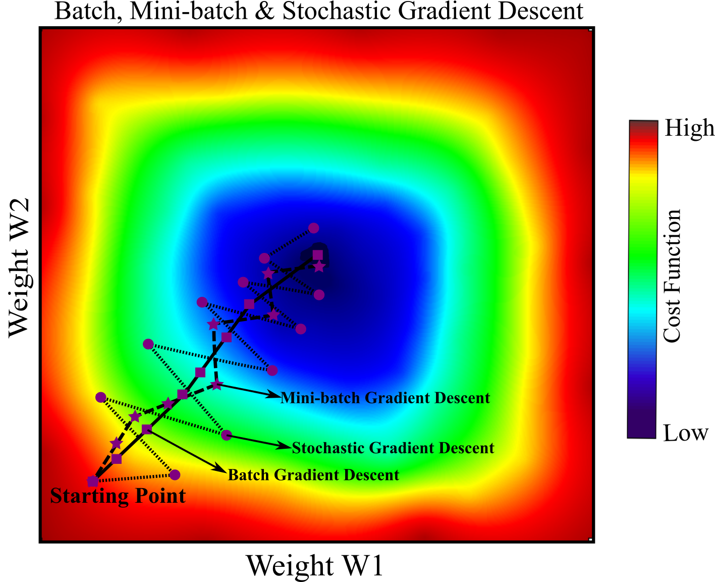
Figure below shows a 2D schematic illustration of paths taken by Batch, Mini-batch and Stochastic Gradient Descent. They all end up near the minimum, but the path for Batch Gradient Descent stops at the minimum, while both Stochastic and Mini-batch continue to walk around. However, it must be noted again that Batch Gradient Descent takes a lot of time for each step. If you have a large data set, it may be efficient to apply Batch Gradient Descent; moreover there is high possibility to get stuck in local minimum. Mini-batch and Stochastic Gradient Descent would reach the global minimum, if you use a good learning schedule, with much less possibility of getting stuck in local minimum.
Polynomial Regression
All examples presented before are simple linear models, but what about non-linear correlation. It is possible to apply a linear model to fit nonlinear data. A simple technique is to add each feature's power as new features, then a linear model is trained on the new features. This approach is called Polynomial Regression. The following code shows how to generate a non-linear second degree polynomial data using a quadratic equation adding some noise.
fig = plt.subplots(figsize=(20,4), dpi= 100, facecolor='w')

ax1=plt.subplot(1,3,1)
np.random.seed(32)
X =8 * np.random.rand(200, 1)-3                 # Generate random numbers from a Uniform distribution
y = -0.4* X**2 +1.5*X+ 5+np.random.randn(200, 1)   # Add random noise from a Uniform distribution
plt.plot(X,y,'ro')
plt.title("Nonlinear Correlation",fontsize=13)
plt.xlabel("X",fontsize=15)
plt.ylabel("y",fontsize=15)

plt.show()
We can use PolynomialFeatures class of Scikit-Learn to apply a polynomial regression. First, the square of each feature as new feature is added to the data set; then a linear model is fitted to the features.
from sklearn.preprocessing import PolynomialFeatures

features_poly = PolynomialFeatures(degree=2, include_bias=False)
Poly_X = features_poly.fit_transform(X)   # Add a square of each feature to data set
Poly_X has the square of X feature plus the original feature. A LinearRegression model can be now fitted to this training data (square and original feature):
lin_reg = LinearRegression()
lin_reg.fit(Poly_X, y)

print( 'w0: ',lin_reg.intercept_[0])
print( 'w1: ',lin_reg.coef_[0][0])
print( 'w2: ',lin_reg.coef_[0][1])
The original function is $-0.40X^{2}+1.50X+5.0$+ Gaussian noise. The predicted function is $-0.40X^{2}+1.53X+4.99$ that is quite similar to the original function. Lets fit the predicted model (blue line) to the data set (red dots):
fig = plt.subplots(figsize=(20,4), dpi= 100, facecolor='w')

ax1=plt.subplot(1,3,1)
New_X=np.linspace(-3, 5, 200).reshape(200, 1)
Poly_New_X = features_poly.transform(New_X)
y_pre = lin_reg.predict(Poly_New_X)
plt.plot(X,y,'ro')
plt.plot(New_X,y_pre,'b-',linewidth=3,label='Predicted Model')
plt.title("Polynomial Regression Model Prediction",fontsize=13)
plt.xlabel("X",fontsize=15)
plt.ylabel("y",fontsize=15)
plt.legend(loc=4, fontsize=12)
plt.show()
Overfitting and Underfitting
The predicted model shown in last Figure is 2-degree Polynomial model that generalizes the data set very well. If 1-degree Polynomial Regression is performed, the training data will not fit well. If higher-degree Polynomial Regression is applied, the training data will be fit much better than with plain Linear Regression. However, both 1-degree and higher than 2-degree Polynomial Regression should not be reliable. The following code shows fitted linear model (1-degree) and 25-degree Polynomial model compared and 2-degree Polynomial model.
fig = plt.subplots(figsize=(20,4), dpi= 100, facecolor='w')

ax1=plt.subplot(1,3,1)

degree=[1,2,25]
width=[2,4,4]
style=["k+-","b--","g-"]
text=['Underfitting: ','Generalized: ','Overfitting  : ']
plt.plot(X, y, "ro", linewidth=3)
for i in range(3):
    features_poly = PolynomialFeatures(degree=degree[i], include_bias=False)
    Poly_X = features_poly.fit_transform(X)
    lin_reg = LinearRegression()
    lin_reg.fit(Poly_X, y)
    Poly_New_X = features_poly.transform(New_X)
    y_pre = lin_reg.predict(Poly_New_X)
    plt.plot(New_X, y_pre, style[i], label=text[i]+str(degree[i])+'- Degree', linewidth=width[i])

plt.xlabel("X",fontsize=15)
plt.ylabel("y",fontsize=15)
plt.title('Underfitting, Generalized and Overfitting Models')
plt.legend(loc=4, fontsize=12)
plt.axis([-3, 5, -4, 8])
plt.show()
The plain Linear Regression (1-degree) is severely underfitting the training set, and 25-degree Polynomial Regression is overfitting. We can see that the best generalized model is the quadratic model. We choose a the quadratic model since we generated the synthetic data with that but in practice we will not know that the data is generated using what function. So, how we can select complexity of a model to make sure it is neither overfitting nor underfitting the data? We talked in previous lectures, how to use cross validation to estimate the performance of model (generalization performance). The model is overfitting if it performs well on the training set but generalizes poorly according to the cross-validation metric.
Another approach to recognize if a model is overfitting or underfitting is look at the learning curves discussed in Aurélien Géron, 2019. We can make plots of model performance for both training set and validation set versus training size. The size of training set gradually increases and we can monitor model performance.
from sklearn.metrics import mean_squared_error
from sklearn.model_selection import train_test_split

def Learning_Curves_Plot(degree,X, y):
    X_training, X_validation, y_training, y_validation = train_test_split(X, y, test_size=0.2,random_state=30)
    training_errors, validation_errors = [], []
    for n in range(1, len(X_training)):
        features_poly = PolynomialFeatures(degree=degree, include_bias=False)
        Poly_X_training   = features_poly.fit_transform(X_training[:n])
        Poly_X_validation = features_poly.fit_transform(X_validation)
        lin_reg = LinearRegression()
        lin_reg.fit(Poly_X_training, y_training[:n])
        y_training_predict   = lin_reg.predict(Poly_X_training)
        y_validation_predict = lin_reg.predict(Poly_X_validation)
        training_errors.append(mean_squared_error(y_training[:n], y_training_predict))
        validation_errors.append(mean_squared_error(y_validation, y_validation_predict))
    plt.plot(training_errors, "b-", linewidth=2, label="Training set")
    plt.plot(validation_errors, "r-+", linewidth=3, label="Validation set")
    plt.xlabel("Training size",fontsize=13)
    plt.ylabel("MSE",fontsize=13)
    plt.legend(loc=1)
Lets apply a linear model (degree=1):
fig = plt.subplots(figsize=(5,3.5), dpi= 100, facecolor='w')
lin_reg = LinearRegression()
degree=1
Learning_Curves_Plot(degree,X, y)
plt.title("Learning Curves_Underfitting",fontsize=14)
plt.ylim((0, 8))
plt.show()
Lets explain above plot. We start with small training size. When there are only one or two instances, the model can perfectly fit them and the MSE for training set will be zero. But when we increase number of training, it is impossible to achieve perfect fit because of increasing noisy in training data. So the MSE in training set gradually increases until it reaches to a point that by increasing training size MSE does not change that much and settles to a plateau. But the curve is completely different for validation set. MSE for Validation set is initially very high because the model is incapable of of generalizing well using very few training instances. Then by increasing the training size, the model learns better and MSE for Validation set slowly goes down. However, since we use a linear model (degree=1) it is severely underfitting because of low performance for both training and validation set: reaching to a plateau at the end. We should use a more complex model.
The following code applies 25-degree polynomial model:
fig = plt.subplots(figsize=(5,3.5), dpi= 100, facecolor='w')
lin_reg = LinearRegression()
degree=25
Learning_Curves_Plot(degree,X, y)
plt.title("Learning Curves_Overfitting",fontsize=14)
plt.ylim((0, 20))
plt.show()
25-degree polynomial model is clearly overfitting because we have very low MSE for training set but very high MSE for validation set.
Finally we try 2-degree polynomial model that best generalized data below:
fig = plt.subplots(figsize=(5,3.5), dpi= 100, facecolor='w')
lin_reg = LinearRegression()
degree=2
Learning_Curves_Plot(degree,X, y)
plt.title("Learning Curves_Generalized",fontsize=14)
plt.ylim((0, 8))
plt.show()
2-degree is generalized much better. First, the MSE is much lower than with the 1-degree (Linear Regression) (underfitting). Second, the gap between the curves is smaller compared with 25-degree model (overfitting).
Understanding of the Bias/Variance Tradeoff
A model's total error can be broken down as the sum of three very different errors:
$Total\,Error=Bias^{2}+Variance+Irreducible\,Error$
- $Bias$
This error happens because of wrong assumptions. For example, if you have a nonlinear data but you assume the data is linear. Underfiting the training data is most likely due to the high error bias.
- $Variance$
We should expect higher variance in prediction if we use a complex model for example a high-degree polynomial model so it overfits the training data. On the contrary, a simple model leads to lower variance. This error happens because of the model's high sensitivity to small variations in the training data.
- $Irreducible error$
This error is because of the noisiness of the data. In order to reduce this part of the error, the data should be cleaned: noise, error and artifact, should be removed before feed Machine Learning algorithms. This error cannot be reduced by Machine Learning algorithms. It can only be reduced by better data cleaning.
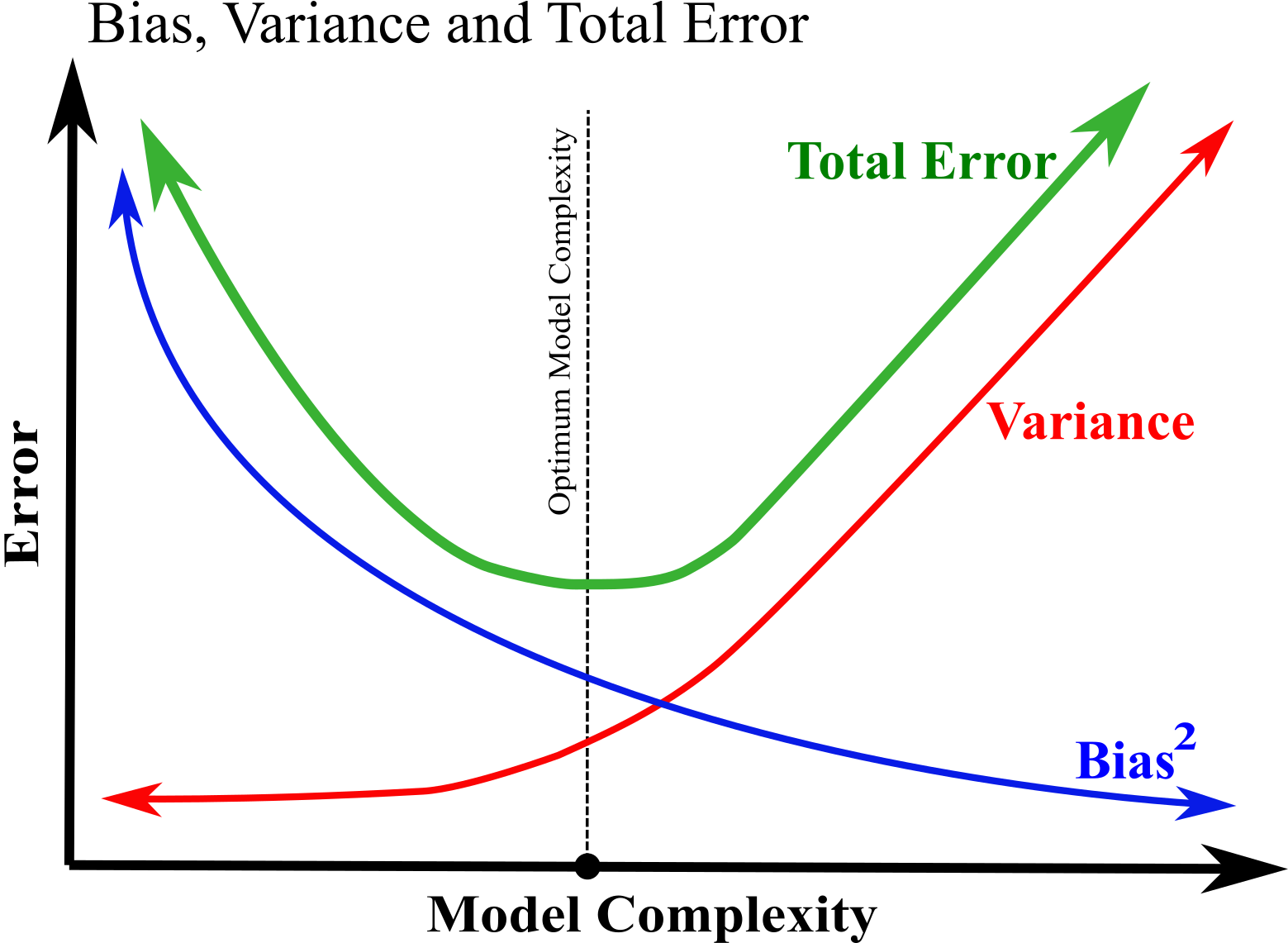
The reason why it is called the Bias/Variance Tradeoff because increasing model complexity should increase the variance and reduce bias error. The opposite is by reducing a complexity of a model its variance reduces but its bias increases. An optimum model should keep a balance of bias and variance error; it should lead to a model that is neither overfit nor underfit. See the Figure below:
Reduce Overfitting
As we saw earlier, a good way to reduce overfitting is to use a less complex model. However, there are other techniques to reduce overfitting and using a complex model at the same time. One approach is regularization. For a linear model, this technique constrains the weights of the model. We will discuss Ridge and Lasso regularization. Another technique to avoid overfitting is early stopping that end iteration (epoch) before starts overfitting. See more information about the following techniques to reduce overfitting.
Ridge (L2 Regularization)
Ridge Regression (also called Tikhonov/L2 regularization) is a regularized version of Linear Regression: a term $\frac{\alpha}{2} \sum_{i=1}^{n}\mathbf{w}_{i}^{2}$ is added to the cost function. Since the cost function should be minimized, the higher $\alpha$, the higher regularization. If $\alpha$ is high, then all weights will receive values close to zeros. If $\alpha=0$, no regularization will be applied. Regularization should only be applied for training. The evaluation of the model should be performed without regularization. In the meantime, regularization does not apply for $w_{0}$. The Ridge Regression cost function is calculated as:
$MSE(\mathbf{w})+ \frac{\alpha}{2} \sum_{i=1}^{n}\mathbf{w}_{i}^{2}$
It is important to scale the data before applying Ridge Regression.
import numpy as np

np.random.seed(42)
n = 30
X = 3.2 * np.random.rand(n, 1)
y = 0.95 + 0.7 * X + np.random.randn(n, 1) / 1.65
X_new = np.linspace(0, 3.2, 100).reshape(100, 1)
Here is the code to apply Ridge Regularization for linear regression
from sklearn.linear_model import Ridge
ridge_reg = Ridge(alpha=1, random_state=42)  # Using a matrix factorization technique by Cholesky
ridge_reg.fit(X, y)
ridge_reg.predict([[3.2]])
Here is another code to apply Ridge Regularization using Stochastic Gradient Descent.
reg_sgd = SGDRegressor(penalty="l2", random_state=42)
reg_sgd.fit(X, y.ravel())
reg_sgd.predict([[3.2]])
Stochastic Gradient Decent use the penalty hyperparameter for regularization: "l2" is Ridge Regularization.
The following function implement Ridge Regularization for a linear model on left and for a 10-degree polynomial regression:
from sklearn.preprocessing import StandardScaler
from sklearn.linear_model import Ridge

def plot_model(model_class, degree, alphas):
    style=["r-", "g-+", "b--"]
    for i in range(3):
        features_poly = PolynomialFeatures(degree=degree, include_bias=False)
        Poly_X   = features_poly.fit_transform(X)
        scaler = StandardScaler()
        Poly_X_Std=scaler.fit_transform(Poly_X)
        lin_reg = Ridge(alpha=alphas[i], solver="cholesky", random_state=42)
        lin_reg.fit(Poly_X_Std, y)
        y_predict = lin_reg.predict(Poly_X_Std)

        Poly_X_new = features_poly.fit_transform(X_new)
        Poly_X_new_Std=scaler.fit_transform(Poly_X_new)
        y_new_regul = lin_reg.predict(Poly_X_new_Std)

        plt.plot(X_new, y_new_regul, style[i], linewidth=1.5, label=r"$\alpha = $"+str(alphas[i]))
    plt.plot(X, y, "ro", linewidth=3,markersize=4)
    plt.legend(loc=2, fontsize=11)
    plt.xlabel('X', fontsize=14)
    plt.ylabel('y', fontsize=14)
    plt.axis([0, 3.2, 0, 4])
fig = plt.subplots(figsize=(10,3.5), dpi= 100, facecolor='w')

plt.subplot(121)
plot_model(Ridge, degree=1, alphas=[0, 25, 10000])
plt.title("Ridge Regularization for Linear Model ",fontsize=13)

plt.subplot(122)
plot_model(Ridge, degree=10, alphas=[0, 10**-4, 0.9])
plt.title("Ridge Regularization for Polynomial Model ",fontsize=13)

plt.show()
As you can see, by increasing $\alpha$, the curves tend to flatter that means they get less extreme, and more reliable predictions are achieved. The variance of the model is reduced but bias increases.
Lasso (L1 Regularization)
Lasso or L1 Regularization is another regularization technique of Linear Regression; similar to Ridge it adds a regularization term to the cost function, which is sum of absolute values of weights:
$MSE(\mathbf{w})+\alpha \sum_{i=1}^{n}|\mathbf{w}_{i}|$
Lasso completely removes the weights for the features that are the least important (the values of the weights set to zero). So, feature selection can be automatically applied by Lasso Regularization.
You should use L1 regularization when you are concerned about low weight values. The lower weight values will typically lead to less overfitting. Generally L2 regularization will produce better overall performance than L1. However, as it was mentioned, L1 might be useful in situations where we have a large number of features and we want to remove some of the weaker inputs (feature selection).
The following code shows how to apply Lasso regularization in Sickit-learn:
from sklearn.linear_model import Lasso
reg_lasso = Lasso(alpha=0.1)
reg_lasso.fit(X, y)
reg_lasso.predict(X[:3])
Elastic Net
The ElasticNet regression is a combination of both L1 and L2 (a L1 + b L2). Both penalties are applied. See the equation below. If r = 0 in equation below, Elastic Net is the same as Ridge Regression, and if r = 1, Elastic Net is equivalent to Lasso Regression.
$MSE(\mathbf{w})+r\alpha \sum_{i=1}^{n}|\mathbf{w}_{i}|+ \frac{1-r}{2} \alpha\sum_{i=1}^{n}\mathbf{w}_{i}^{2}$
The following code shows how to implement Elastic Net using Scikit-Learn:
from sklearn.linear_model import ElasticNet
r=0.5
ela_net = ElasticNet(alpha=0.2, l1_ratio=r)
ela_net.fit(X, y)
ela_net.predict([[3.2]])
So the question is which regularization technique (Ridge, Lasso, or Elastic Net) we should use? or is it required to have any regularization? In general, it is recommended to have a little regularization. Generally the performance of L2 (Ridge) regularization is better than L1 regularization (Lasso). So, L2 regularization is a good default. However, if you believe that only a few features are actually useful, you can apply Lasso or Elastic Net because they convert the weights of the useless features to zero. Elastic Net is generally preferred over Lasso because if some features are strongly correlated or the number of features are greater than the number of training instances Lasso may behave randomly Aurélien Géron, 2019. All these regularization are applied for Neural Network.
Early Stopping
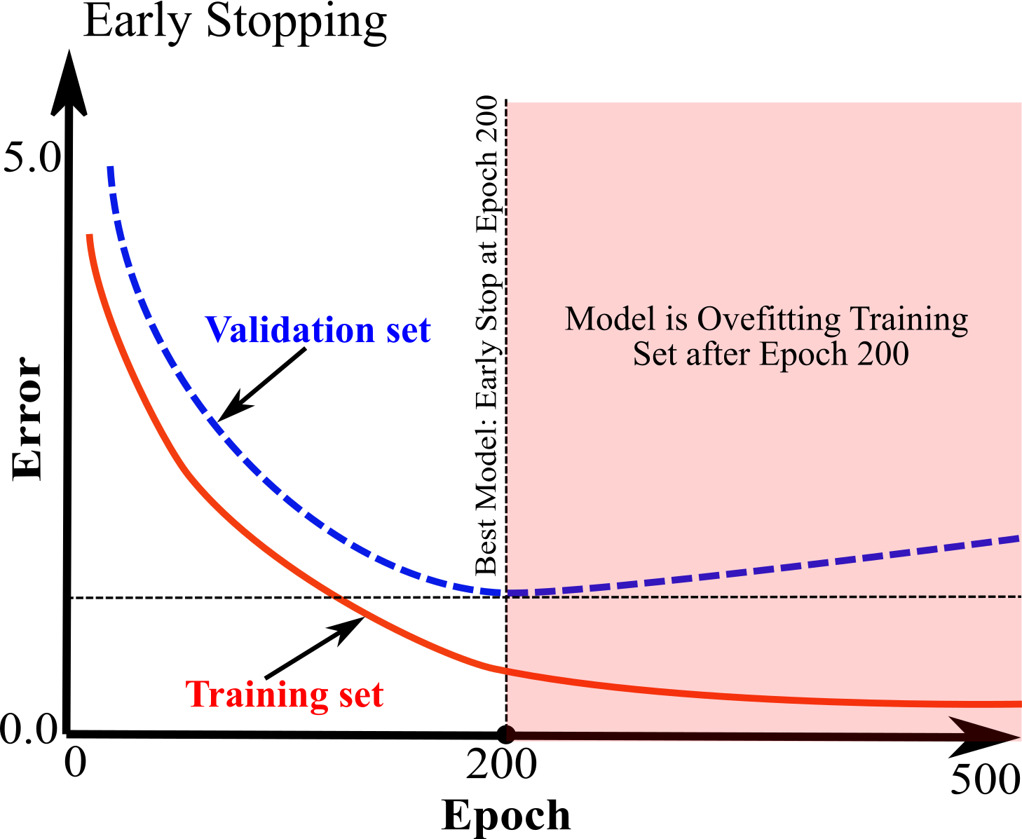
Early stoping is a very useful and different technique for regularization to avoid overfitting. It works for iterative algorithms; it stops iteration once the error for validation set reaches to a minimum and just starts to increase while the error for training set keeps decreasing. Figure below shows a schematic illustration of early stopping for Batch Gradient Descent. Number of iteration call Epoch. You can see before Epoch 200, error in both training and validation decrease; at Epoch 200 we have minimum error for validation set, but after that, error is going to increase for validation set while error in training set keeps decreasing. This indicates that after Epoch 200 models starts to overfit the training set so the iteration should be stopped at Epoch 200. Although this approach is very simple, it is a very efficient regularization technique. It is such a simple and efficient regularization technique that Geoffrey Hinton called it a beautiful free lunch.
Logistic Regression
We discussed some algorithms that can be used for both regression and classification. Logistic Regression (or Logit Regression) is a technique applied to estimate the probability of an instance belonging to a class. For example probability of a email being Spam. If the probability is bigger than 0.5 (or 50%), it predicts the instance as a positive class (label 1) or if less than 0.5, it predicts the instance as negative class (label 0). That is why it is called a binary classification.
Probability Estimation
The question is how logistic regression estimates the probability. It works similar to linear regression by calculating the weighted sum of input features plus a bias or intercept term; however, unlike linear regression that outputs the result directly, logistic regression output the result after applying a Sigmoid Function:
$\large \bar{p}=S(\mathbf{x}^{T}\mathbf{w})$
where $S$ is a Sigmoid Function that is a S-shaped function. The output of Sigmoid Function is always between 0 and 1. The Equation below shows Sigmoid Function:
$\large S(t)=\frac{1}{1+e^{-t}}$
fig = plt.subplots(figsize=(7,3.5), dpi= 100, facecolor='w')

t = np.linspace(-5, 5, 100)
S = 1 / (1 + np.exp(-t))

plt.plot(t, S, "r-", linewidth=3, label=r"$S(t) = \frac{1}{1 + e^{-t}}$")
plt.plot([-5, 5], [0, 0], "k-")
plt.plot([-5, 5], [0.5, 0.5], "k--")
plt.plot([-5, 5], [1, 1], "k--")
plt.plot([0, 0], [-1.1, 1.1], "k-")
plt.axis([-5, 5, 0, 1.1])
plt.xlabel("t", fontsize=14)
plt.ylabel("Probability "+ r'($\bar{p}$)', fontsize=14)
plt.title("Logistic Regression", fontsize=16)
plt.legend(loc=4, fontsize=14)

plt.show()
Logistic Regression predicts a model based on the calculated probability: predict 0 (y=0) probability less than 0.5 and predict 1 (y=1) for probability bigger than 0.5:
$\bar{p}=\left\{\begin{matrix} if\,\,\bar{p}<0.5 \,\,\,\,\,\,\,\, 0 \\ \\ if\,\,\bar{p}\geq 0.5 \,\,\,\,\,\,\,\, 1 \end{matrix}\right. $
Cost Function and Training Model
We saw how Logistic Regression works. The question is how the probabilities are estimated with Logistic Regression. This requires model training and minimizing a cost function to calculate optimum weights $\mathbf{w}$ in Equation below
$\large \bar{p}=\frac{1}{1+e^{-\mathbf{x}^{T}\mathbf{w}}}$
Where $\mathbf{x}$ is the vector of features. For each instance, the model should predict the class 1 with high probability (y=1) and class 0 with low probability (y=0); so a cost function $C$ for a single instance can be represented as:
$C=\left\{\begin{matrix} if\,\,y=1 \,\,\,\,\,\,\,\,\,\, -log(\bar{p}) \\ \\ \,\,\,\,if\,\,y=0 \,\,\,\,\,\,\, -log(1-\bar{p}) \end{matrix}\right.$
$C$ is a reasonable cost function because if y=1, we should have $\bar{p}=1$ for a perfect prediction. By decreasing $\bar{p}$, we will have higher error since $-log(\bar{p})$ increases as $\bar{p}$ decreases. On the other hand, if y=0, we should have $\bar{p}=0$ for a perfect prediction. By increasing $\bar{p}$, we will have higher error since $-log(1-\bar{p})$ increases as $\bar{p}$ goes up.
The average cost over all training instances can be written as a single expression below that is called log loss:
$C=-\frac{1}{n}\sum_{i=1}^{n}\begin{pmatrix} (y_{i})log (\bar{p}_{i})+(1-y_{i})log(1-\bar{p}_{i}) \end{pmatrix}$
There is no know equation for calculating the optimized $\mathbf{w}$ by minimizing this cost function (the Normal Equation). Fortunately the cost function is convex, thus Gradient Descent can find the optimum weights that minimizes the cost function. Remember how gradient descent works:
$\Large w=w-\alpha \frac{\partial C}{\partial w}$
So we only need to calculate the partial derivative of $C$ with regards to each weight. This derivative is achieved as:
$\large\frac{\partial C}{\partial w_{j}}=\frac{1}{n}\sum_{i=1}^{n}(\frac{1}{1+e^{-\mathbf{w}^{T}x^{(i)}}}-y^{(i)})x^{(i)}_{j}$
See here for the proof of this derivative. For each instance the prediction error is calculated and multiplied it by the $j_{th}$ feature value, and then it computes the average over all training instances. You can simply use the Batch Gradient Descent algorithm when you have the gradient vector for all partial derivatives. That is how training for logistic regression works. As we discussed before, Batch Gradient Descent uses all training instances; Mini-batch uses a mini-batch at a time and Stochastic takes one instance at a time.
The following code shows how generate a synthetic data with two class (0 and 1) and then apply logistic regression.
np.random.seed(50)
X = np.random.rand(200, 2) - 0.5
y = (X[:, 0] > 0).astype(np.float32)
def rotate(x0,y0,x,y,Ang):
    """Rotate coordinate"""
    import math
    xa=[]
    ya=[]
    Angle=Ang *(math.pi/180)
    for i in range(len(x)):
        tmp1=x[i]-x0
        tmp2=y[i]-y0
        X=(tmp2)*math.sin(Angle)+(tmp1)*math.cos(Angle)
        xa.append(X+x0)
        Y=(tmp2)*math.cos(Angle)-(tmp1)*math.sin(Angle)
        ya.append(Y+y0)
    xa=np.array(xa).reshape(len(xa),1)
    ya=np.array(ya).reshape(len(ya),1)
    X=np.concatenate((xa,ya),axis=1)
    return X
from matplotlib.colors import ListedColormap
import matplotlib
import matplotlib.pyplot as plt

font = {'size'   : 12}
matplotlib.rc('font', **font)
fig = plt.subplots(figsize=(6.0, 4.5), dpi= 90, facecolor='w', edgecolor='k')

X=rotate(0,0,X[:, 0],X[:, 1],-45)
plt.plot(X[:, 0][y==0], X[:, 1][y==0], "bs", label="Class 0")
plt.plot(X[:, 0][y==1], X[:, 1][y==1], "r^", label="Class 1")

plt.axis([-0.75, 0.75, -0.75, 0.75])
plt.xlabel(r"$X_{1}$", fontsize=18)
plt.ylabel(r"$X_{2}$", fontsize=18, rotation=0)

plt.legend(loc=2, fontsize=14)
plt.show()
The below fit a Logistic Regression to classify 0 and class for the entire domain.
from sklearn.linear_model import LogisticRegression
log_reg = LogisticRegression(random_state=42)
log_reg.fit(X, y)
from matplotlib.path import Path
from matplotlib.patches import PathPatch
def clip_domain():
    """ Clip prediction"""
    path=(0,-0.75),(-0.75,-0.75),(-0.75,0),(0,-0.75),(-0.75,0),(-0.75,0.75),(0,0.75),(-0.75,0)
    path1 = np.asarray(path)
    path2 = Path(path1)
    patch = PathPatch(path2, facecolor='w',linewidth=0)
    plt.gca().add_patch(patch)

    path=(0,0.75),(0.75,0),(0.75,0.75),(0,0.75),(0,-0.75),(0.75,-0.75),(0.75,0),(0,-0.75)
    path1 = np.asarray(path)
    path2 = Path(path1)
    patch = PathPatch(path2, facecolor='w',linewidth=0)
    plt.gca().add_patch(patch)
    plt.xlim((-0.75, 0.75))
    plt.ylim((-0.75, 0.75))
    plt.show()
font = {'size'   : 12}
matplotlib.rc('font', **font)
fig = plt.subplots(figsize=(6.0, 4.5), dpi= 90, facecolor='w', edgecolor='k')

x1s = np.linspace(-0.75,0.75, 100)
x2s = np.linspace(-0.75,0.75, 100)
x1, x2 = np.meshgrid(x1s, x2s)
X_new = np.c_[x1.ravel(), x2.ravel()]
y_pred = log_reg.predict(X_new).reshape(x1.shape)

custom_cmap = ListedColormap(['b','r'])
plt.contourf(x1, x2, y_pred, alpha=0.3, cmap=custom_cmap)

plt.plot(X[:, 0][y==0], X[:, 1][y==0], "bs", label="Class 0")
plt.plot(X[:, 0][y==1], X[:, 1][y==1], "r^", label="Class 1")

plt.axis([-0.75, 0.75, -0.75, 0.75])
plt.xlabel(r"$X_{1}$", fontsize=18)
plt.ylabel(r"$X_{2}$", fontsize=18, rotation=0)
plt.legend(loc=2, fontsize=14)
clip_domain()
plt.show()
Softmax Regression
The Logistic Regression model can be applied to classify multiple classes directly. This is called Softmax Regression. The Softmax Regression model first calculates a score sk(x) for each class k, then estimates the probability of each class by applying the softmax function to the scores. The Softmax score instance x for each class is calculated by:
$z_{k}=\boldsymbol{\mathbf{}x}^{T}\mathbf{w}^{(k)}$
When the score of every class for the instance x is calculated, the probability belongs to class k can be estimated by the Softmax function below which calculates the the exponential of every score then divides by the sum of all the exponentials:
$\large p_{k}=S(z_{k})=\frac{e^{z_{k}}}{\sum_{i=1}^{K}(e^{z_{i}})}$
Lets make a synthetic data set with three classes and then apply Softmax Regression.
np.random.seed(50)
X = np.random.rand(500, 2) - 0.5
y = []
for i in list(X[:, 0]):
    if(i<=-0.15):
        y.append(0)
    if(i>-0.15 and i<0.15):
        y.append(1)
    if(i>0.15):
        y.append(2)
y=np.array(y)
font = {'size'   : 12}
matplotlib.rc('font', **font)
fig = plt.subplots(figsize=(6.0, 4.5), dpi= 90, facecolor='w', edgecolor='k')

X=rotate(0,0,X[:, 0],X[:, 1],-45)
plt.plot(X[:, 0][y==0], X[:, 1][y==0], "bs", label="Class 0")
plt.plot(X[:, 0][y==1], X[:, 1][y==1], "r^", label="Class 1")
plt.plot(X[:, 0][y==2], X[:, 1][y==2], "go", label="Class 2")

plt.axis([-0.75, 0.75, -0.75, 0.75])
plt.xlabel(r"$X_{1}$", fontsize=18)
plt.ylabel(r"$X_{2}$", fontsize=18, rotation=0)

plt.legend(loc=3, fontsize=14)
plt.show()
softmax_reg = LogisticRegression(multi_class="multinomial", random_state=42)
softmax_reg.fit(X, y)
font = {'size'   : 12}
matplotlib.rc('font', **font)
fig = plt.subplots(figsize=(6.0, 4.5), dpi= 90, facecolor='w', edgecolor='k')

x1s = np.linspace(-0.75,0.75, 100)
x2s = np.linspace(-0.75,0.75, 100)
x1, x2 = np.meshgrid(x1s, x2s)
X_new = np.c_[x1.ravel(), x2.ravel()]
y_pred = softmax_reg.predict(X_new).reshape(x1.shape)
custom_cmap = ListedColormap(['b','r'])
plt.contourf(x1, x2, y_pred, alpha=0.3, cmap=custom_cmap)

plt.plot(X[:, 0][y==0], X[:, 1][y==0], "bs", label="Class 0")
plt.plot(X[:, 0][y==1], X[:, 1][y==1], "r^", label="Class 1")
plt.plot(X[:, 0][y==2], X[:, 1][y==2], "go", label="Class 2")

plt.axis([-0.75, 0.75, -0.75, 0.75])
plt.xlabel(r"$X_{1}$", fontsize=18)
plt.ylabel(r"$X_{2}$", fontsize=18, rotation=0)

plt.legend(loc=3, fontsize=14)
clip_domain()
plt.show()